Andrew W. Trask's Blog

One plausible description for "the goal of the AI community" goes like this: to build automated systems which solve all of humanity's problems both now and in the future. Surely our lives would be better if our problems were solved? This goal natural follows from a related observation: nearly all of humanity is in some way taking part in helping to solve humanity's present or future problems. This is what we're all doing, so wouldn't it be great if AI could do it all for us? Bonus points if it can solve all our problems better than we can!

An interesting tangent is to observe that if we simply had more humans to help we would make faster progress on solving humanity's problems. However, adding more humans also makes many of the problems harder (hunger, war, global warming, etc.). Thus, it's important to consider that some plausible solutions to "all of humanity's problems" are net-negative in their approach, causing more problems than they fix. But beyond observing that net-nevative solutions exist, and that AI-related solutions could be net-negative too, let's set this aside for the moment.

For anyone else who also learned AI from Russell and Norvig's influential book, it's often useful to think about AI form the perspective of a database and a search algorithm. If your live-updating database contains the answer to any question, and you have enough compute to query it fast enough, then you have AGI and in theory all of humanity's problems are solved. Pick any problem, ask for the solution, and do it. This could be high level questions ("What is the meaning of life?") or low-level questions ("Should my car turn 3 degrees to the left?"), but as long as they're all in the database then you're good.

However, no such database exists for a multitude of reasons, such as:

we don't have that much data collected anywhere, or the means to collect it if we did have that much data, we wouldn't have enough compute even if we had enough compute, we wouldn't have enough energy to run that compute

That is to say, from this perspective, solving AGI is mostly about efficiency. We can group efficiency into useful groups such as:

Information re-use (generalization, convolution, shared weights, etc.): learning something once in one area and then re-using it elsewherex. information priority (attention, regularization, etc.): being able to know when information is simply irrelevant to you and not worth encoding or propagating at all (such as random noise, or parts of an image that simply aren't relevant to the task at hand).

So if the ultimate fallback towards AGI is just data collection (memorization, like in a database), AI is trying to give us more efficient methods than simply collecting everything under the sun. Information re-use and prioritization schemes are plausibly the most popular strategies.

In short - we live in a world of finite resources, so solving AGI is actually about saying "How far can we get with the smallest amount of "x" resource?" Given fixed supply, whomever can be the most efficient can be the most intelligent. In a world with limited energy, efficiency is intelligence.

So what type of AGI will be the most intelligent? Hive-mind or single-model?

First, let's define the difference:

Single-model: a model wherein a large group of parameters are always entirely used for every prediction. Hive-mind: a group of models wherein only models which are relevant to a problem are used to make a prediction.

So for example, single-model AGI would encode all of the world's information into one giant "blob" of parameters. This would include information about chess, checkers, romantic relationships, klingon curse words, nuclear launch codes, brownie baking instructions, and the number of freckles on your dead gradmother's right earlobe.

But a hive-mind AGI would separate each of these discplines into sub-models dedicated to each specific area. There might be a recipes model, a dating model, a proliferation model, etc. And while they could certainly communicate with each other if necessary, they are under no obligation to. Meaning the overal system is organized into these distinct groups, subsets of which are only activated if the topic at hand is relevant to them.

Note that whether something is a single-model or hive-mind AGI is totally orthogonal to whether the model is running on a single compute system owned by a single organization. A hive-mind could all be run by one corporation, and a single-model could be co-run by many corporations. This is largely orthogonal, although it's probably easier to decentralize governance over a hive-mind, but that's not what this post is about.

The key premise is this - if we buy the id that efficiency is intelligence, the hive-mind style of AGI should (in the long run) strongly out-compete single-model AGI on every intelligence task it faces. Why? Because it doesn't need to activate parameters on totally irrelevant tasks. And because it's using inforamtion more efficiently, it can outperform other models which were using information less efficiently.

Put another way, if it takes 100 billion parameters to do one weight update and learn one paragraph of a recipe book, you're not going to learn as many recipes as the model which can do the same with 100 million parameters focused exclusively on cooking. The latter will simply learn way more recipes a lot faster.

Now, it's essential that the hive-mind be able to share inforamtion across specialty areas. And the AI community really hasn't cracked this approach yet which is why single-model (massive models) seem to be doing so well. But if we zoom out and look at ML fundamentals, this advantage will probably be short-lived. Models are going to have specialized sub-components. Single-model approaches might be winning a couple battles, but hive-minds will win the war.

Related:

superhuman models on board games aren't trained on medical tasks, and there's little to indicate doing so would be helpful to the board game performance. superhuman models on medical tasks aren't trained on driving cars, and there's little to indicate that being able to drive better would help one with medical tasks. governance and safety is probably easier if AGI ownership is actually spread amongst a large number of different entities for the same reason that democracy is better than totalitarianism. And while this is doable for single-model AI, it's probably a lot easier for hive-mind AI.

TLDR: I've recently wondered about whether the Universe is truly random, and I thought I'd write down a few thoughts on the subject. As a heads up, this post is more about sharing a personal journey I'm on than teaching a skill or tool (unlike many other blogposts). Feel free to chat with me about these ideas on Twitter as I'm still working through them myself and I'd love to hear your perspective.

I typically tweet out new blogposts when they're complete @iamtrask. Thank you for your time and attention, and I hope you enjoy the post.

The Oxford English Dictionary defines randomness as "a lack of pattern or predictability in events". I like this definition as it reveals that "randomness" is more about the predictive ability of the observer than about an event itself. Consider the following consequence of this definition:

Consequence: Two people can accurately describe the same event as having different degrees of randomness.

Consider when two meterologists are trying to predict the probability that it will rain today. One person (we will call them the "Ignorant Meterologist") is only allowed a record of how often it has rained in the region between the years 1900 and 2000. The second person (the "Smart Meterologist") is also allowed this information, but this second individual is also allowed to know today's date. These two individuals would consider the likelihood of rain to be very different. The Ignorant Meterologist would simply say, "it rains 40% of the time in the region, thus there is a 40% chance of rain today.". What else can he/she say? Given the information provided, the degree of randomness is very high. However, the "Smart Meterologist" is more informed. He/she might be able to say "it is the dry season, thus there is only a 5% chance of rain today".

If we asked each of these meterologists to continue to make predictions over time. They would each make predictions with different degrees of randomness (one higher and one lower) in accordance with the availability of information. However, the event is no more or less random in and of itself. It's only more or less random in relation to an invidual and other available predictive information.

Perhaps this makes you feel that randomness is no longer real, that it is only in the eye of the beholder. However, I believe that the context of Machine Learning provides a much more precise definition of randomness. In this context, one can think of randomness as a measure of compatability between 3 datasets: "input", "target", and "model".

Input: is data that is readily known. It is what we're going to try to use to predict something else. All potential "causes" are contained within the input.

Target: is the data that we wish to predict. This is the thing that we say is either random or not random.

Model: this "dataset" is simply a set of instructions for transforming the input into the target. When a human is making a prediction, this is the human's intelligence. In a computer, it's a large series of 1s and 0s which operate gates and represent a particular transformation.

Thus, we can view randomness as merely a degree of compatability between these three datasets. If there is a high degree of compatability (input -> model -> target is very reliable), then there is a low degree of randomness.

Now that we've identified what I believe to be the most practical and commonly used definition of randomness, I'd like to introduce the bigger version of randomness, which we'll call Randomness (with a capital R). This Randomness refers to whether, given infinite knowledge and intelligence, a future event could be predicted before it happens (a "model" dataset could exist for that event). This Randomness also implies whether or not something is caused by another thing. If it is NOT caused but simply IS of its own accord, it is (capital "R") Random.

Is the Universe Random?

The simple answer is that, from our perspective, it has a degree of randomness that is rapidly decreasing. We are consistently able to predict future events with greater accuracy. Furthermore, predicting outcomes given our interaction allows us a certain degree of control over the future (because we can choose interactions which we predict will lead to the desired outcome). This plays out in the advancement of every sector: agriculture, healthcare, finance (bigtime), politics, etc. However, because we cannot predict the Universe entirely, it is somewhat random. (lowercase "r")

Whether the Universe is uppercase "R" Random is a different question entirely. We can, however, make some progress on this question:

Claim 1: Causality exists

In short, we can predict things with far better than random accuracy. Thus, some things tend to cause other things. We might even be able to say that some things absolutely cause other things unless effected by some unpredictable randomness, but we don't even need this bold of a claim. Simply stated, much of the Universe is probably causal because we can predict events with better than random accuracy. To claim otherwise would be extremely unlikely and would imply that the entirety of human innovation and intelligence throughout history leading to prosperity and survival was simply a coincidence. It's possible, but very unlikely. We'll go ahead and accept the notion that causality exists in the Universe.

Claim 2: The Universe is not entirely Random.

For all things in the Universe that are not Random but are instead caused, randomness (lowercase) in their behavior is a result of either random or Random objects exerting upon it. Thus, asking whether the Universe is Random is about asking whether or not there exists a Random object within it. It is not about asking whether every object is inherently random, because cause and effect can transfer the unpredictable behavior of a Random object across the Universe via things that are merely random.

Claim 3: Because we can observe cause and effect relationships, the Universe is, at most, a mixture of Random and causal objects, and at least, exclusively made of causal objects.

This brings us to the root of our question. When we repeatedly ask "and what caused that?" over and over again, where do we end up? Well, there are 4 possible states of the Universe (finite/finite space/time)

Finite Time + Finite Space If time is finite, there was a beginning. If there was a beginning, there was a TON of Randomness which began the Universe. Thus, Randomness at least has existed within the Universe (although whether it still exists is less certain).
Finite Time + Infinite Space (see above)
Infinite Time + Finite Space Laws of entropy determine that if this was our Universe, you wouldn't be reading this blogpost as all the energy in the Universe would have disipated to equilibrium an infinite number of years ago. I suppose there are counter arguments to this, but I don't personally find them particularly strong. We have a rather large amount of empirical evidence that energy tends to dissipate (perhaps more empirical evidence for this than for any other claim in the Universe?).
Infinite Time + Infinite Space This state is interesting because there's theoretically an infinite amount of energy (inside the infinite space) alongside an infinite amount of time for it to disipate. Thus, while I don't have solid footing to say that this Universe does not exist, I think we can make a reasonble case for (capital R) Randomness in this Universe. Specifically, because the state of the Universe at any given time "t" is, itself, infinite, there are an infinite number of potential causes for an event. Thus, every event is Random because there are an infinite number of potential causes for any event. It may be asymtotically predicatable given proximity to some causal events playing a more dominant role, but in the limit every event is Random.

Conclusion: Randomness with a capital R either exists or has existed before in the Universe because all 3 plausible configurations of the Universe necessitate events that have no cause, and an event with no cause cannot be predicted and is therefore Random.

TLDR: What if it was possible for surveillance to only invade the privacy of criminals or terrorists, leaving the innocent unsurveilled? This post proposes a way with a prototype in Python.

Abstract: Modern criminals and terrorists hide amongst the patterns of innocent civilians, exactly mirroring daily life until the very last moments before becoming lethal, which can happen as quickly as a car turning onto a sidewalk or a man pulling out a knife on the street. As police intervention of an instantly lethal event is impossible, law enforcement has turned to prediction based on the surveillance of public and private data streams, facilitated by legislation like the Patriot Act, USA Freedom Act, and the UK's Counter-Terrorism Act. This legislation sparks a heated debate (and rightly so) on the tradeoff between privacy and security. In this blogpost, we explore whether much of this tradeoff between privacy and security is merely a technological limitation, overcommable by a combination of Homomorphic Encryption and Deep Learning. We supplement this discussion with a tutorial for a working prototype implementation and further analysis on where technological investments could be made to mature this technology. I am optimistic that it is possible to re-imagine the tools of crime prediction such that, relative to where we find ourselves today, citizen privacy is increased, surveillance is more effective, and the potential for mis-use is mitigated via modern techniques for Encrypted Artificial Intelligence.

Edit:The term "Prediction" seemed to trigger the assumption that I was proposing technology to predict "future" crimes. However, it was only intended to describe a system that can detect crime unfolding (including intent / pre-meditation) in accordance with agreed upon defintions of "intent" and "pre-meditation" in our criminal justice system, which do relate to future crimes. However, I am in no way advocating punishment for people who have commited no crime. So, I'm changing the title to "Detection" to better communicate this.

Edit 2: Some have critiqued this post by citing court cases when tools such as drug dogs or machine learning have been either inaccurate or biased based on unsuitable characteristics such as race. These constitute fixable defects in the predictive technology and have little to no bearing on this post. This post is, instead, about how homomorphic encryption can allow this technology to run out in the open (on private data), the nature of which does NOT constitute a search or seizure because it reveals no information about any citizen other than whether or not they are commiting a crime (much like a drug dog giving your bag a sniff. It knows everything in your bag but doesn't tell anyone. It only informs the public whether or not you are likely committing a crime... triggering a search or seizure.) Ways to make the underlying technology more accurate can be discussed elsewhere.

Edit 3: Others have critiqued this post by confusing it with tech for allocation of police resources, which uses high level statistical informaiton to basically predict "this is a bad neighborhood". Note that tech such as this is categorically different than what I am proposing, as it makes judgements against large groups of people, many of whom have committed no crime. This technology is instead about detecting when crimes actually occur but would normally go un-discovered because no information to the crime's existence was made public (i.e., the "perfect crime").

I typically tweet out new blogposts when they're complete @iamtrask. If these ideas inspire you to help in some way, a share or upvote is the first place to start as a lack of awareness of these tools is the greatest obstacle at this stage. All in all, thank you for your time and attention, and I hope you enjoy the post.

Part 1: Ideal Citizen Surveillance

When you are collecting your bags at an international airport, often a drug sniffing dog will come up and give your bag a whiff. Amazingly, drug dogs are trained to detect conceiled criminal activity with absolutely no invasion of your privacy. Before drug dogs, enforcing the same laws required opening up every bag and searching its contents looking for drugs, an expensive, time consuming, privacy invading procedure. However, with a drug dog, the only bags that need to be searched are those that actually contain drugs (according to the dog). Thus, the development of K9 narcotics units simultaneously increased the privacy, effectiveness, and efficiency of narcotics surveillance.

Source:http://www.vivapets.com/upload/Image/...

Similarly, in much of the developed world it is a commonly accepted practice to install an electronic fire alarm or burgular alarm in one's home. This first wave of the Internet of Things constitutes a voluntary, selective invasion of privacy. It is a piece of intelligence that is designed to only invade our privacy (and inform home security phone operators or law enforcement to the state of your doors and windows and give them permission to enter your home) if there is a great need for it (a threat to life or property such as a fire or burgular). Just like drug dogs, fire alarms and burgular alarms replace a much less efficient, far more invasive, expensive system: a guard or fire watchman standing at your house 24x7. Just like drug dugs, fire alarms and burgular alarams simultaneously incrase privacy, effectiveness, and efficiency of home surveillance.

In these two scenarios, there is almost no detectable tradeoff between privacy and security. It is a non-issue as a result of technological solutions that filter through irrelevant, invasive information to only detect the rare bits of information indicative of a crime or a threat to life or property. This is the ideal state of surveillance. Surveillance is effective yet privacy is protected. This state is reachable as a result of several characteristics of these devices:

Privacy is only invaded if danger/criminal activity is highly probable.
The devices are accurate, with a low occurrence of False Positives.
Those with access to the device (homeowners and K9 handlers) aren't explicitly trying to fool it. Thus, its inner workings can be made public, allowing it's protection of privacy to be fully known / auditable (no need for self-regulation of alarm manufacturers or dog handlers)

This combination of privacy protection, accuracy, and auditability is the key to the ideal state of surveillance, and it's quite intuitive. Why should every bag be opened and every airline passenger's privacy violated when less than 0.001% will actually contain drugs? Why should video feeds into people's homes be watched by security guards when 99.999% of the time there is no invasion or fire? More precisely, should it even be possible for a surveillance state to surveil the innocent, presenting the opportunity for corruption? Is it possible to create this limit to a surveillance state's powers while simultaneously increasing its effectiveness and reducing cost? What would such a technology look like? These are the questions explored below.

Part 2: National Security Surveillance

At the time of writing, over 50 people have been killed by terror attacks in the last two weeks alone in Manchester, London, Egypt, and Afghanistan. My prayers go out to the victims and their families, and I deeply hope that we can find more effective ways to keep people safe. I am also reminded of the recent terror attack in Westminster, which claimed the lives of 4 people and injured over 50. The investigation into the attack in Westminster revealed that it was coordinated on WhatsApp. This has revived a heated debate on the tradeoff between privacy and safety. Governments want back-doors into apps like WhatsApp (which constitute unrestricted READ access to a live data stream), but many are concerned about trusting big brother to self-regulate the privacy of WhatsApp users. Furthermore, installing open backdoors makes these apps vulnerable to criminials discovering and exploiting them, further increasing risks to the public. This is reflective of the modern surveillance state.

Privacy is only violated as a means to an end of detecting extremely rare events (attacks)
There's a high degree of false positives in data collection (presumably 99.9999% of the data has nothing to do with an actual threat).
If the detection technology was released to the public, presumbly bad actors would seek to evade it. Thus, it has to be deployed in secret behind a firewall (not auditable). This opens up the opportunity for mis-use (although in most nations I personally believe misuse is rare).

These three characteristics of national surveillance states are in stark contrast to the three ideal characteristics mentioned in the introduction. There is largely believed to be significant collateral damage to the privacy of innocent bystanders in data streams being surveilled. This is a result of the detection technology needing to remain secret. Unlike drug dogs, algorithms used to find bad actors (terrorists, criminals, etc.) can't be deployed (i.e. on WhatsApp) out in public for everyone to see and audit for privacy protection. If they were released to the public to be evaluated for privacy protection they would quickly be reverse engineered and their effects deemed useless. Furthermore, even deploying them to people's phones (without auditing) to detect criminal activity would constitute a vulnerability. Bad actors would evade the algorithms by reverse engineering them and by vieweing/intercepting/faking their predictions being sent back to the state. Instead, entire data streams must be re-directed to warehouses for stockpiling and analysis, as it is impossible to determine which subsets of the data stream are actually relevant using an automatic method out in public.

While terrorism is perhaps the most discussed domain in the tradeoff between privacy and safety, it is not the only one. Crimes such as murder take the lives of hundreds of thousands of individuals around the world. The US alone averages around 16,000 murders per year, which oddly can be abstracted to a logistical issue: Law enforcement does not know of a crime far enough in advance to intervene. On average, 16,000 Americans simply call 911 too late, if they manage to call at all.

The Chicken and Egg Problem of "Probable Cause": The challenge faced by the FBI and local law enforcement is incredibly similar to that of terrorism. The laws intended to protect citizens from the invasive nature of surveillance create a chicken and egg problem between observing "probable cause" for a crime (subsequently obtaining a warrant), and having access to the information indicative of "probable cause" in the first place. Thus, unless victims can somehow know (predict) they are about to be murdered far enough in advanced to send out a public cry for help, law enforcement is often unable to prevent their death. Viewing crime prediction from this light is an interesting perspective, as it moves crime prediction from something a citizien must invoke for themselves to a public good that justifies public funding and support.

Bottom line: the cost of this chicken-and-egg "probable cause" issue is not only the invasion of citizen privacy, it is an extremely large number of human lives owing to the inability for people to predict when they will be harmed far enough in advance for law enforcement to intervene. Dialing 911 is often too little, too late. However, in rare cases like drug dogs or fire alarms, this is a non-issue as crime is detectable without significant collateral damage to privacy and thus "probable cause" is no longer a limiting factor to keeing the public safe.

Part 3: The Role of Artificial Intelligence

In a perfect world, there would be a "Fire Alarm" device for activities involving irreversible, heinous crimes such as assault, murder, or terrorism, that was private, accurate, and auditable. Fortunately, the R&D investment into devices for this kind of detection by commerical entities has been massive. To be clear, this investment hasn't been driven by the desire for consumer privacy. On the contrary, these devices were developed to achieve scale. Consider developing Gmail and wanting to offer a feature that filters out SPAM. You could invade people's privacy and read all their emails by hand, but it would be faster and cheaper to build a machine that can simply detect SPAM such that you can filter through hundreds of millions of emails per day with a few dozen machines. Given that law enforcement seeks to protect such a large population (presumably filtering through rather massive amounts of data looking for criminals/terrorists), it is not hard to expect that there's a high degree of automation in this process. Bottom line, narrow AI based automation is probably involved. So, given this assumption, what we really lack is an ability to transform our AI agents such that:

they can be audited by a trusted party for privacy protection
they can't be reverse engineered when deployed
their predictions can't be known by those being surveilled
their predictions can't be falsified by the deploying party (such as a chat application)
reasonably efficient and scalable

In order to fully define this idea, we will be building a prototype "Fire Detector" for crime. In the next section, we're going to build a basic version of this detector using a 2 layer neural network. After that, we're going to upgrade this detector so that it meets the requirements listed above. For the sake of exposition, this detector is going to be trained on a SPAM dataset and thus will only detect SPAM, but it could conceivably be trained to detect any particular event you wanted (i.e., murder, arson, etc.). I only chose SPAM because it's relatively easy to train and gives me a simple, high quality network with which to demonstrate the methods of this blogpost. However, the spectrum of possible detectors is as broad as the field of AI itself.


Part 4: Building a SPAM Detector

So, our demo use case is that a local law enforcement officer (we'll call him "Bob") is hoping to crack down on people sending out SPAM emails. However, instead of reading everyone's emails, Bob only wants to detect when someone is sending SPAM so that he can file for an injunction and acquire a warrant with the police to further investigate. The first part of this process is to simply build an effective SPAM detector.

The Enron Spam Dataset: In order to teach an algorithm how to detect SPAM, we need a large set of emails that has been previously labeled as "SPAM" or "NOT SPAM". That way, our algorithm can study the dataset and learn to tell the difference between the two kinds of emails. Fortunately, a prominent energy company called Enron committed a few crimes recorded in email, and as a result a rather large subset of the company's emails were made public. As many of these were SPAM, a dataset was curated specifically for building SPAM detectors called the Enron Spam Dataset. I have further pre-processed this dataset for you in the following files: HAM and
SPAM. Each line contains an email. There are 22,032 HAM emails, and 9,000 SPAM emails. We're going to set aside the last 1,000 in each category as our "test" dataset. We'll train on the rest.

The Model: For this model, we're going to optimize for speed and simplicity and use a simple bag-of-words Logistic Classifier. It's a neural network with 2 layers (input and output). We could get more sophisticated with an LSTM, but this blogpost isn't about filtering SPAM, it's about making surveillance less intrusive, more accountable, and more effective. Besides that, bag-of-words LR works really well for SPAM detection anyway (and for a surprisingly large number of other tasks as well). No need to overcomplicate. Below you'll find the code to build this classifier. If you're unsure how this works, feel free to review my previous post on A Neural Network in 11 Lines of Python.

(fwiw, this code works identically in Python 2 or 3 on my machine)



import numpy as np
from collections import Counter
import random
import sys

np.random.seed(12345)

f = open('spam.txt','r')
raw = f.readlines()
f.close()

spam = list()
for row in raw:
spam.append(row[:-2].split(" "))

f = open('ham.txt','r')
raw = f.readlines()
f.close()

ham = list()
for row in raw:
ham.append(row[:-2].split(" "))

class LogisticRegression(object):

def __init__(self, positives,negatives,iterations=10,alpha=0.1):

# create vocabulary (real world use case would add a few million
# other terms as well from a big internet scrape)
cnts = Counter()
for email in (positives negatives):
for word in email:
cnts[word] = 1

# convert to lookup table
vocab = list(cnts.keys())
self.word2index = {}
for i,word in enumerate(vocab):
self.word2index[word] = i

# initialize decrypted weights
self.weights = (np.random.rand(len(vocab)) - 0.5) * 0.1

# train model on unencrypted information
self.train(positives,negatives,iterations=iterations,alpha=alpha)

def train(self,positives,negatives,iterations=10,alpha=0.1):

for iter in range(iterations):
error = 0
n = 0
for i in range(max(len(positives),len(negatives))):

error = np.abs(self.learn(positives[i % len(positives)],1,alpha))
error = np.abs(self.learn(negatives[i % len(negatives)],0,alpha))
n = 2

print("Iter:" str(iter) " Loss:" str(error / float(n)))


def softmax(self,x):
return 1/(1 np.exp(-x))

def predict(self,email):
pred = 0
for word in email:
pred = self.weights[self.word2index[word]]
pred = self.softmax(pred)
return pred

def learn(self,email,target,alpha):
pred = self.predict(email)
delta = (pred - target)# * pred * (1 - pred)
for word in email:
self.weights[self.word2index[word]] -= delta * alpha
return delta

model = LogisticRegression(spam[0:-1000],ham[0:-1000],iterations=3)

# evaluate on holdout set

fp = 0
tn = 0
tp = 0
fn = 0

for i,h in enumerate(ham[-1000:]):
pred = model.predict(h)

if(pred < 0.5):
tn = 1
else:
fp = 1

if(i % 10 == 0):
sys.stdout.write('\rI:' str(tn tp fn fp) " % Correct:" str(100*tn/float(tn fp))[0:6])

for i,h in enumerate(spam[-1000:]):
pred = model.predict(h)

if(pred >= 0.5):
tp = 1
else:
fn = 1

if(i % 10 == 0):
sys.stdout.write('\rI:' str(tn tp fn fp) " % Correct:" str(100*(tn tp)/float(tn tp fn fp))[0:6])
sys.stdout.write('\rI:' str(tn tp fn fp) " Correct: %" str(100*(tn tp)/float(tn tp fn fp))[0:6])

print("\nTest Accuracy: %" str(100*(tn tp)/float(tn tp fn fp))[0:6])
print("False Positives: %" str(100*fp/float(tp fp))[0:4] " <- privacy violation level out of 100.0%")
print("False Negatives: %" str(100*fn/float(tn fn))[0:4] " <- security risk level out of 100.0%")





Iter:0 Loss:0.0455724486216
Iter:1 Loss:0.0173317643148
Iter:2 Loss:0.0113520767678
I:2000 Correct: .798
Test Accuracy: .7
False Positives: %0.3 <- privacy violation level out of 100.0%
False Negatives: %0.3 <- security risk level out of 100.0%

Feature: Auditability: a nice feature of our classifier is that it is a highly auditable algorithm. Not only does it give us accurate scores on the testing data, but we can open it up and look at how it weights various terms to make sure it's flagging emails based on what officer Bob is specifically looking for. It is with these insights that officer Bob seeks permission from his superior to perform his very limited surveillance over the email clients in his jurisdiction. Note, Bob has no access to read anyone's emails. He only has access to detect exactly what he's looking for. The purpose of this model is to be a measure of "probable cause", which Bob's superior can make the final call on given the privacy and security levels indicated above for this model.

Ok, so we have our classifier and Bob gets it approved by his boss (the chief of police?). Presumably, law enforcement officer "Bob" would hand this over to all the email clients within his jurisdiction. Each email client would then use the classifier to make a prediction each time it's about to send an email (commit a crime). This prediction gets sent to Bob, and eventually he figures out who has been anonymously sending out 10,000 SPAM emails every day within his jurisdiction.

Problem 1: His Predictions Get Faked - after 1 week of running his algorithm in everyone's email clients, everyone is still receiving tons of SPAM. However, Bob's Logistic Regression Classifier apparently isn't flagging ANY of it, even though it seems to work when he tests some of the missed SPAM on the classifier with his own machine. He suspects that someone is intercepting the algorithm's predictions and faking them to look like they're all "Negative". What's he to do?

Problem 2: His Model is Reverse Enginered - Furthermore, he notices that he can take his pre-trained model and sort it by its weight values, yielding the following result.

While this was advantageous for auditability (making the case to Bob's boss that this model is going to find only the information it's supposed to), it makes it vulnerable to attacks! So not only can people intercept and modify his model's predictions, but they can even reverse engineer the system to figure out which words to avoid. In other words, the model's capabilities and predictions are vulnerable to attack. Bob needs another line of defense.

Part 5: Homomorphic Encryption

In my previous blogpost Building Safe A.I., I outlined how one can train Neural Networks in an encrypted state (on data that is not encrypted) using Homomorphic Encryption. Along the way, I discussed how Homomorphic Encryption generally works and provided an implementation of Efficient Integer Vector Homomorphic Encryption with tooling for neural networks based on this implementation. However, as mentioned in the post, there are many homomorphic encryption schemes to choose from. In this post, we're going to use a different one called Paillier Cryptography, which is a probabilistic, assymetric algorithm for public key cryptography. While a complete breakdown of this cryptosystem is something best saved for a different blogpost, I did fork and update a python library for paillier to be able to handle larger cyphertexts and plaintexts (longs) as well as a small bugfix in the logging here Paillier Cryptosystem Library. Pull that repo down, run "python setup.py install" and try out the following code.

As you can see, we can encrypt (positive or negative) numbers using a public key and then add their encrypted values together. We can then decrypt the resulting number which returns the output of whatever math operations we performed. Pretty cool, eh? We can use just these operations to encrypt our Logistic Regression classifier after training. For more on how this works, check out my previous post on the subject, otherwise let's jump straight into the implementation.



import phe as paillier
import math
import numpy as np
from collections import Counter
import random
import sys

np.random.seed(12345)

print("Generating paillier keypair")
pubkey, prikey = paillier.generate_paillier_keypair(n_length=64)

print("Importing dataset from disk...")
f = open('spam.txt','r')
raw = f.readlines()
f.close()

spam = list()
for row in raw:
spam.append(row[:-2].split(" "))

f = open('ham.txt','r')
raw = f.readlines()
f.close()

ham = list()
for row in raw:
ham.append(row[:-2].split(" "))

class HomomorphicLogisticRegression(object):

def __init__(self, positives,negatives,iterations=10,alpha=0.1):

self.encrypted=False
self.maxweight=10

# create vocabulary (real world use case would add a few million
# other terms as well from a big internet scrape)
cnts = Counter()
for email in (positives negatives):
for word in email:
cnts[word] = 1

# convert to lookup table
vocab = list(cnts.keys())
self.word2index = {}
for i,word in enumerate(vocab):
self.word2index[word] = i

# initialize decrypted weights
self.weights = (np.random.rand(len(vocab)) - 0.5) * 0.1

# train model on unencrypted information
self.train(positives,negatives,iterations=iterations,alpha=alpha)



def train(self,positives,negatives,iterations=10,alpha=0.1):

for iter in range(iterations):
error = 0
n = 0
for i in range(max(len(positives),len(negatives))):

error = np.abs(self.learn(positives[i % len(positives)],1,alpha))
error = np.abs(self.learn(negatives[i % len(negatives)],0,alpha))
n = 2

print("Iter:" str(iter) " Loss:" str(error / float(n)))


def softmax(self,x):
return 1/(1 np.exp(-x))

def encrypt(self,pubkey,scaling_factor=1000):
if(not self.encrypted):
self.pubkey = pubkey
self.scaling_factor = float(scaling_factor)
self.encrypted_weights = list()

for weight in model.weights:
self.encrypted_weights.append(self.pubkey.encrypt(\\
int(min(weight,self.maxweight) * self.scaling_factor)))

self.encrypted = True
self.weights = None


return self

def predict(self,email):
if(self.encrypted):
return self.encrypted_predict(email)
else:
return self.unencrypted_predict(email)

def encrypted_predict(self,email):
pred = self.pubkey.encrypt(0)
for word in email:
pred = self.encrypted_weights[self.word2index[word]]
return pred

def unencrypted_predict(self,email):
pred = 0
for word in email:
pred = self.weights[self.word2index[word]]
pred = self.softmax(pred)
return pred

def learn(self,email,target,alpha):
pred = self.predict(email)
delta = (pred - target)# * pred * (1 - pred)
for word in email:
self.weights[self.word2index[word]] -= delta * alpha
return delta

model = HomomorphicLogisticRegression(spam[0:-1000],ham[0:-1000],iterations=10)

encrypted_model = model.encrypt(pubkey)

# generate encrypted predictions. Then decrypt them and evaluate.

fp = 0
tn = 0
tp = 0
fn = 0

for i,h in enumerate(ham[-1000:]):
encrypted_pred = encrypted_model.predict(h)
try:
pred = prikey.decrypt(encrypted_pred) / encrypted_model.scaling_factor
if(pred < 0):
tn = 1
else:
fp = 1
except:
print("overflow")

if(i % 10 == 0):
sys.stdout.write('\r I:' str(tn tp fn fp) " % Correct:" str(100*tn/float(tn fp))[0:6])

for i,h in enumerate(spam[-1000:]):
encrypted_pred = encrypted_model.predict(h)
try:
pred = prikey.decrypt(encrypted_pred) / encrypted_model.scaling_factor
if(pred > 0):
tp = 1
else:
fn = 1
except:
print("overflow")

if(i % 10 == 0):
sys.stdout.write('\r I:' str(tn tp fn fp) " % Correct:" str(100*(tn tp)/float(tn tp fn fp))[0:6])
sys.stdout.write('\r I:' str(tn tp fn fp) " % Correct:" str(100*(tn tp)/float(tn tp fn fp))[0:6])

print("\n Encrypted Accuracy: %" str(100*(tn tp)/float(tn tp fn fp))[0:6])
print("False Positives: %" str(100*fp/float(tp fp))[0:4] " <- privacy violation level")
print("False Negatives: %" str(100*fn/float(tn fn))[0:4] " <- security risk level")




Generating paillier keypair
Importing dataset from disk...
Iter:0 Loss:0.0455724486216
Iter:1 Loss:0.0173317643148
Iter:2 Loss:0.0113520767678
Iter:3 Loss:0.00455875940625
Iter:4 Loss:0.00178564065045
Iter:5 Loss:0.000854385076612
Iter:6 Loss:0.000417669805378
Iter:7 Loss:0.000298985174998
Iter:8 Loss:0.000244521525096
Iter:9 Loss:0.000211014087681
I:2000 % Correct:99.296
Encrypted Accuracy: .2
False Positives: %0.0 <- privacy violation level
False Negatives: %1.57 <- security risk level

This model is really quite special (and fast!... around 1000 emails per second with a single thread on my laptop). Note that we don't use the sigmoid during prediction (only during training) as it's followed by a threshold at 0.5. Thus, at testing we can simply skip the sigmoid and threshold at 0 (which is identical to running the sigmoid and thresholding at 0.5). However, enough with the technicals, let's get back to Bob.

Bob had a problem with people being able to see his predictions and fake them. However, now all the predictions are encrypted.

Furthermore, Bob had a problem with people reading his weights and reverse engineering how his algorithm had learned to detect. However, now all the weights themselves are also encrypted (and can predict in their encrypted state!).

Now when he deploys his model, no one can read what it is sending to spoof it (or even know what it is supposedly detecting) or reverse engineer it to further avoid its detection. This model has many of the desirable properties that we wanted. It's auditable by a third party, makes encrypted predictions, and its intelligence is also encrypted from those who might want to steal/fool it. Furthermore, it is quite accurate (with no false positives on the testing dataset), and also quite fast. Bob deploys his new model, receives encrypted predictions, and discovers that one particular person seems to be preparing to send out (what the model thinks is) 10,000 suspiciously SPAMY emails. He reports the metric to his boss and a judge, obtains a warrant, and rids the world of SPAM forever!!!!

Part 6: Building Safe Crime Prediction

Let's take a second and consider the high level difference that this model can make for law enforcement. Present day, in order to detect events such as a murder or terrorist attack, law enforcement needs unrestricted access to data streams which might be predictive of the event. Thus, in order to detect an event that may occur in 0.0001% of the data, they have to have access to 100% of the data stream by re-directing it to a secret warehouse wherein (I assume) Machine Learning models are likely deployed.

However, with this approach the same Machine Learning models currently used to identify crimes can instead be encrypted and used as detectors which are deployed to the data stream itself (i.e., chat applications). Law Enforcement then only has access to the predictions of the model as opposed to having access to the entire dataset. This is similar to the use of drug dogs in an airport. Drug dogs eliminate the need for law enforcement to search everyone's bags looking for cocaine. Instead, a dog is TRAINED (just like a Machine Learning model) to exclusively detect the existence of narcotics. Barking == drugs. No barking == no drugs. POSITIVE neural network prediction means "a terrorist plot is being planned on this phone", NEGATIVE neural network prediction means "a terrorist plot is NOT being planned on this phone". Law enforcement has no need to see the data. They only need this one datapoint. Furthermore, as the model is a discrete piece of intelligence, it can be independently evaluated to ensure that it only detects what it's supposed to (just like we can independently audit what a drug dog is trained to detect by evaluating the dog's accuracy through tests). However, unlike drug dogs, Encrypted Artificial Intelligence could provide this ability for any crime that is detectable through digitial evidence.

Auditing Concerns: So, who do we trust to perform the auditing? I'm not a political science expert, so I'll leave this for others to comment. However, I think that third party watchdogs, a mixture of government contractors, or perhaps even open source developers could perform this role. If there are enough versions of every detector, it would likely be very difficult for bad actors to figure out which one was being deployed against them (since they're encrypted). I see several plausible options here and, largely, auditing bodies over government organizations seems like the kind of problem that many people have thought about before me, so I'll leave this part for the experts. ;)

Ethical Concerns: Notably, literary work provides commentary around the ethical and moral implications of crime predictions leading to a conviction directly, (such as in the 1956 short story "Minority Report", the origin of the term "precrime"). However, the primary value of crime prediction is not efficient punishment and inprisonment, it's the prevention of harm. Accordingly, there are two trivial ways to avoid this moral dilemma. First, the vast majority of crimes require smaller crimes in advance of a larger one (i.e., conspiracy to commit), and simply predicting the larger crime by being able to more accurately detect the smaller crimes of preparation avoids much of the moral dilemma. Secondly, pre-crime technology can simply be used as a method for how to best allocate police resources as well as a method for triggering a warrant/investigation (such as Bob did in our example). This latter use inparticular is perhaps the best use of crime prediction technology if the privacy security tradeoff can be mitigated (the topic of this blogpost). A positive prediction should launch an investigation, not put someone behind bars directly.

Legal Concerns: United States v. Place ruled that because drug dogs are able to exclusively detect the odor of narcotics (without detecting anything else), they are not considered a "search". In other words, because they are able to classify only the crime without requiring a citizen to divulge any other information, it is not considered an invasion of privacy. Furthermore, I believe that the general feeling of the public around this issue reflects the law. A fluffy dog coming up and giving your rolling bag a quick sniff at the airport is a very effective yet privacy preserving form of surveillance. Curiously, the dog un-doubtedly could be trained to detect the presence of any number of embarassing things in your bag. However, it is only TRAINED to detect those indicative of a crime. In the same way, Artificial Intelligence agents can be TRAINED to detect signs indicative of a crime without detecting anything else. As such, for models that achieve a sufficiently high accuracy rate, these models could obtain a similar legal status as drug dogs.

Authoritarian Corruption Concerns: Perhaps you're wondering, "Why innovate in this space? Why propose new methods for surveillance? Aren't we being surveilled enough?". My answer is this: It should be impossible for those who do NOT harm one another (the innocent) to be surveilled by corporations or governments. Inversely, we want to detect anyone about to injure another human far enough in advance to stop them. Before recent technological advancements, these two statements were clearly impossible to achieve together. The purpose of this blogpost is to make one point: I believe it is technologically plausible to have both perfect safety and perfect privacy. By "perfect privacy", I mean privacy that is NOT subject to the whims of an authoritarian government, but is instead limited by auditable technology like Encrypted Artificial Intelligence. Who should be responsible for auditing this technology without revealing its techniques to bad actors? I'm not sure. Perhaps it's 3rd party watchdog organizations. Perhaps it's instead a system people opt-in to (like Fire Alarms) and there's a social contract established such that people can avoid those who do not opt in (because... why would you?). Perhaps it's developed entirely in the open source but is simply so effective that it can't be circumvented? These are some good questions to explore in subsequent discussions. This blogpost is not the whole solution. Social and government structures would undoubtedly need to adjust to the advent of this kind of tool. However, I do believe it is a significant piece of the puzzle, and I look forward to the conversations it can inspire.


Part 7: Future Work

First and foremost, we need modern float vector Homomorphic Encryption algorithms (FV, YASHE, etc.) supported in a major Deep Learning framework (PyTorch, Tensorflow, Keras, etc.). Furthermore, exploring how we can increase the speed and security of these algorithms is an actively innovated and vitally important line of work. Finally, we need to imagine how social structures could best partner with these new tools to protect people's safety without violating privacy (and continue to reduce the risk of authoritarian governments misusing the technology).

Part 8: Let's Talk

At the end of May, I had the pleasure of meeting with the brilliant Carrick Flynn and a number of wonderful folks from the Future of Humanity Institute, one of the world's leading labs on A.I. Safety. We were speaking as they have recently become curious about Homomorphic Encryption, especially in the context of Deep Learning and A.I. One of the use cases we explored over Indian cuisine was that of Crime Prediction, and this blogpost is an early derivative of our conversation (hopefully one of many). I hope you find these ideas as exciting as I do, and I encourage you to reach out to Carrick, myself, and FHI if you are further curious about this topic or the Existential Risks of A.I. more broadly. To that end, if you find yourself excited about the idea that these tools might reduce government surveillance down to only criminals and terrorists, don't just click on! Help spread the word! (upvote, share, etc.) Also, I'm particularly interested in hearing from you if you work in one of several industries (or can make introductions):

Law Enforcement: I'm very curious as to the extent to which these kinds of tools could become usable, particularly for local law enforcement. What are the major barriers to entry to tools such as these becoming useful for the triggering of a warrant? What kinds of certifications are needed? Do you know of similar precedent/cases? (i.e., drug dogs)
DARPA / Intelligence Community / Gov. Contractor: Similar question as for local law enforcement, but with the context being the federal space.
Legislation / Regulation: I envision a future where these tools become mature enough for legislation to be crafted such that they account for improved privacy/security tradeoffs (reduced privacy invasion but expedited warrant triggering procedure). Are there members of the legislative body who are actually interested in backing this type of development?

I typically tweet out new blogposts when they're complete @iamtrask. As mentioned above, if these ideas inspire you to help in some way, a share or upvote is the first place to start as a lack of awareness of these tools is the greatest obstacle at this stage. All in all, thank you for your time and attention, and I hope you enjoyed the post!

Relevant Links


http://blog.fastforwardlabs.com/2017/...
https://eprint.iacr.org/2013/075.pdf
https://iamtrask.github.io/2017/03/17...

TLDR: What if it was possible for surveillance to only invade the privacy of criminals or terrorists, leaving the innocent unsurveilled?

Abstract: Modern criminals and terrorists hide amongst the patterns of innocent civilians, exactly mirroring daily life until the very last moments before becoming lethal, which can happen as quickly as a car turning onto a sidewalk or a man pulling out a knife on the street. As police intervention of an instantly lethal event is impossible, law enforcement has turned to prediction based on the surveillance of public and private data streams, facilitated by legislation like the Patriot Act, USA Freedom Act, and the UK's Counter-Terrorism Act. This legislation sparks a heated debate (and rightly so) on the tradeoff between privacy and security. In this blogpost, we explore whether much of this tradeoff between privacy and security is merely a technological limitation, overcommable by a combination of Homomorphic Encryption and Deep Learning. We supplement this discussion with a tutorial for a working prototype implementation and further analysis on where technological investments could be made to mature this technology. I am optimistic that it is possible to re-imagine the tools of crime prediction such that, relative to where we find ourselves today, citizen privacy is increased, surveillance is more effective, and the potential for mis-use is mitigated via modern techniques for Encrypted Artificial Intelligence.

I typically tweet out new blogposts when they're complete @iamtrask. If these ideas inspire you to help in some way, a share or upvote is the first place to start as a lack of awareness of these tools is the greatest obstacle at this stage. All in all, thank you for your time and attention, and I hope you enjoy the post.

Part 1: Ideal Citizen Surveillance

When you are collecting your bags at an international airport, often a drug sniffing dog will come up and give your bag a whiff. Amazingly, drug dogs are trained to detect conceiled criminal activity with absolutely no invasion of your privacy. Before drug dogs, enforcing the same laws required opening up every bag and searching its contents looking for drugs, an expensive, time consuming, privacy invading procedure. However, with a drug dog, the only bags that need to be searched are those that actually contain drugs (according to the dog). Thus, the development of K9 narcotics units simultaneously increased the privacy, effectiveness, and efficiency of narcotics surveillance.

Source:http://www.vivapets.com/upload/Image/...

Similarly, in much of the developed world it is a commonly accepted practice to install an electronic fire alarm or burgular alarm in one's home. This first wave of the Internet of Things constitutes a voluntary, selective invasion of privacy. It is a piece of intelligence that is designed to only invade our privacy (and inform home security phone operators or law enforcement to the state of your doors and windows and give them permission to enter your home) if there is a great need for it (a threat to life or property such as a fire or burgular). Just like drug dogs, fire alarms and burgular alarms replace a much less efficient, far more invasive, expensive system: a guard or fire watchman standing at your house 24x7. Just like drug dugs, fire alarms and burgular alarams simultaneously incrase privacy, effectiveness, and efficiency of home surveillance.

In these two scenarios, there is almost no detectable tradeoff between privacy and security. It is a non-issue as a result of technological solutions that filter through irrelevant, invasive information to only detect the rare bits of information indicative of a crime or a threat to life or property. This is the ideal state of surveillance. Surveillance is effective yet privacy is protected. This state is reachable as a result of several characteristics of these devices:

Privacy is only invaded if danger/criminal activity is highly probable.
The devices are accurate, with a low occurrence of False Positives.
Those with access to the device (homeowners and K9 handlers) aren't explicitly trying to fool it. Thus, its inner workings can be made public, allowing it's protection of privacy to be fully known / auditable (no need for self-regulation of alarm manufacturers or dog handlers)

This combination of privacy protection, accuracy, and auditability is the key to the ideal state of surveillance, and it's quite intuitive. Why should every bag be opened and every airline passenger's privacy violated when less than 0.001% will actually contain drugs? Why should video feeds into people's homes be watched by security guards when 99.999% of the time there is no invasion or fire? More precisely, should it even be possible for a surveillance state to surveil the innocent, presenting the opportunity for corruption? Is it possible to create this limit to a surveillance state's powers while simultaneously increasing its effectiveness and reducing cost? What would such a technology look like? These are the questions explored below.

Part 2: National Security Surveillance

At the time of writing, over 50 people have been killed by terror attacks in the last two weeks alone in Manchester, London, Egypt, and Afghanistan. My prayers go out to the victims and their families, and I deeply hope that we can find more effective ways to keep people safe. I am also reminded of the recent terror attack in Westminster, which claimed the lives of 4 people and injured over 50. The investigation into the attack in Westminster revealed that it was coordinated on WhatsApp. This has revived a heated debate on the tradeoff between privacy and safety. Governments want back-doors into apps like WhatsApp (which constitute unrestricted READ access to a live data stream), but many are concerned about trusting big brother to self-regulate the privacy of WhatsApp users. Furthermore, installing open backdoors makes these apps vulnerable to criminials discovering and exploiting them, further increasing risks to the public. This is reflective of the modern surveillance state.

Privacy is only violated as a means to an end of detecting extremely rare events (attacks)
There's a high degree of false positives in data collection (presumably 99.9999% of the data has nothing to do with an actual threat).
If the detection technology was released to the public, presumbly bad actors would seek to evade it. Thus, it has to be deployed in secret behind a firewall (not auditable). This opens up the opportunity for mis-use (although in most nations I personally believe misuse is rare).

These three characteristics of national surveillance states are in stark contrast to the three ideal characteristics mentioned in the introduction. There is largely believed to be significant collateral damage to the privacy of innocent bystanders in data streams being surveilled. This is a result of the detection technology needing to remain secret. Unlike drug dogs, algorithms used to find bad actors (terrorists, criminals, etc.) can't be deployed (i.e. on WhatsApp) out in public for everyone to see and audit for privacy protection. If they were released to the public to be evaluated for privacy protection they would quickly be reverse engineered and their effects deemed useless. Furthermore, even deploying them to people's phones (without auditing) to detect criminal activity would constitute a vulnerability. Bad actors would evade the algorithms by reverse engineering them and by vieweing/intercepting/faking their predictions being sent back to the state. Instead, entire data streams must be re-directed to warehouses for stockpiling and analysis, as it is impossible to determine which subsets of the data stream are actually relevant using an automatic method out in public.

While terrorism is perhaps the most discussed domain in the tradeoff between privacy and safety, it is not the only one. Crimes such as murder take the lives of hundreds of thousands of individuals around the world. The US alone averages around 16,000 murders per year, which oddly can be abstracted to a logistical issue: Law enforcement does not know of a crime far enough in advance to intervene. On average, 16,000 Americans simply call 911 too late, if they manage to call at all.

The Chicken and Egg Problem of "Probable Cause": The challenge faced by the FBI and local law enforcement is incredibly similar to that of terrorism. The laws intended to protect citizens from the invasive nature of surveillance create a chicken and egg problem between observing "probable cause" for a crime (subsequently obtaining a warrant), and having access to the information indicative of "probable cause" in the first place. Thus, unless victims can somehow know (predict) they are about to be murdered far enough in advanced to send out a public cry for help, law enforcement is often unable to prevent their death. Viewing crime prediction from this light is an interesting perspective, as it moves crime prediction from something a citizien must invoke for themselves to a public good that justifies public funding and support.

Bottom line: the cost of this chicken-and-egg "probable cause" issue is not only the invasion of citizen privacy, it is an extremely large number of human lives owing to the inability for people to predict when they will be harmed far enough in advance for law enforcement to intervene. Dialing 911 is often too little, too late. However, in rare cases like drug dogs or fire alarms, this is a non-issue as crime is detectable without significant collateral damage to privacy and thus "probable cause" is no longer a limiting factor to keeing the public safe.

Part 3: The Role of Artificial Intelligence

In a perfect world, there would be a "Fire Alarm" device for activities involving irreversible, heinous crimes such as assault, murder, or terrorism, that was private, accurate, and auditable. Fortunately, the R&D investment into devices for this kind of detection by commerical entities has been massive. To be clear, this investment hasn't been driven by the desire for consumer privacy. On the contrary, these devices were developed to achieve scale. Consider developing Gmail and wanting to offer a feature that filters out SPAM. You could invade people's privacy and read all their emails by hand, but it would be faster and cheaper to build a machine that can simply detect SPAM such that you can filter through hundreds of millions of emails per day with a few dozen machines. Given that law enforcement seeks to protect such a large population (presumably filtering through rather massive amounts of data looking for criminals/terrorists), it is not hard to expect that there's a high degree of automation in this process. Bottom line, narrow AI based automation is probably involved. So, given this assumption, what we really lack is an ability to transform our AI agents such that:

they can be audited by a trusted party for privacy protection
they can't be reverse engineered when deployed
their predictions can't be known by those being surveilled
their predictions can't be falsified by the deploying party (such as a chat application)
reasonably efficient and scalable

In order to fully define this idea, we will be building a prototype "Fire Detector" for crime. In the next section, we're going to build a basic version of this detector using a 2 layer neural network. After that, we're going to upgrade this detector so that it meets the requirements listed above. For the sake of exposition, this detector is going to be trained on a SPAM dataset and thus will only detect SPAM, but it could conceivably be trained to detect any particular event you wanted (i.e., murder, arson, etc.). I only chose SPAM because it's relatively easy to train and gives me a simple, high quality network with which to demonstrate the methods of this blogpost. However, the spectrum of possible detectors is as broad as the field of AI itself.


Part 4: Building a SPAM Detector

So, our demo use case is that a local law enforcement officer (we'll call him "Bob") is hoping to crack down on people sending out SPAM emails. However, instead of reading everyone's emails, Bob only wants to detect when someone is sending SPAM so that he can file for an injunction and acquire a warrant with the police to further investigate. The first part of this process is to simply build an effective SPAM detector.

The Enron Spam Dataset: In order to teach an algorithm how to detect SPAM, we need a large set of emails that has been previously labeled as "SPAM" or "NOT SPAM". That way, our algorithm can study the dataset and learn to tell the difference between the two kinds of emails. Fortunately, a prominent energy company called Enron committed a few crimes recorded in email, and as a result a rather large subset of the company's emails were made public. As many of these were SPAM, a dataset was curated specifically for building SPAM detectors called the Enron Spam Dataset. I have further pre-processed this dataset for you in the following files: HAM and
SPAM. Each line contains an email. There are 22,032 HAM emails, and 9,000 SPAM emails. We're going to set aside the last 1,000 in each category as our "test" dataset. We'll train on the rest.

The Model: For this model, we're going to optimize for speed and simplicity and use a simple bag-of-words Logistic Classifier. It's a neural network with 2 layers (input and output). We could get more sophisticated with an LSTM, but this blogpost isn't about filtering SPAM, it's about making surveillance less intrusive, more accountable, and more effective. Besides that, bag-of-words LR works really well for SPAM detection anyway (and for a surprisingly large number of other tasks as well). No need to overcomplicate. Below you'll find the code to build this classifier. If you're unsure how this works, feel free to review my previous post on A Neural Network in 11 Lines of Python.

(fwiw, this code works identically in Python 2 or 3 on my machine)



import numpy as np
from collections import Counter
import random
import sys

np.random.seed(12345)

f = open('spam.txt','r')
raw = f.readlines()
f.close()

spam = list()
for row in raw:
spam.append(row[:-2].split(" "))

f = open('ham.txt','r')
raw = f.readlines()
f.close()

ham = list()
for row in raw:
ham.append(row[:-2].split(" "))

class LogisticRegression(object):

def __init__(self, positives,negatives,iterations=10,alpha=0.1):

# create vocabulary (real world use case would add a few million
# other terms as well from a big internet scrape)
cnts = Counter()
for email in (positives negatives):
for word in email:
cnts[word] = 1

# convert to lookup table
vocab = list(cnts.keys())
self.word2index = {}
for i,word in enumerate(vocab):
self.word2index[word] = i

# initialize decrypted weights
self.weights = (np.random.rand(len(vocab)) - 0.5) * 0.1

# train model on unencrypted information
self.train(positives,negatives,iterations=iterations,alpha=alpha)

def train(self,positives,negatives,iterations=10,alpha=0.1):

for iter in range(iterations):
error = 0
n = 0
for i in range(max(len(positives),len(negatives))):

error = np.abs(self.learn(positives[i % len(positives)],1,alpha))
error = np.abs(self.learn(negatives[i % len(negatives)],0,alpha))
n = 2

print("Iter:" str(iter) " Loss:" str(error / float(n)))


def softmax(self,x):
return 1/(1 np.exp(-x))

def predict(self,email):
pred = 0
for word in email:
pred = self.weights[self.word2index[word]]
pred = self.softmax(pred)
return pred

def learn(self,email,target,alpha):
pred = self.predict(email)
delta = (pred - target)# * pred * (1 - pred)
for word in email:
self.weights[self.word2index[word]] -= delta * alpha
return delta

model = LogisticRegression(spam[0:-1000],ham[0:-1000],iterations=3)

# evaluate on holdout set

fp = 0
tn = 0
tp = 0
fn = 0

for i,h in enumerate(ham[-1000:]):
pred = model.predict(h)

if(pred < 0.5):
tn = 1
else:
fp = 1

if(i % 10 == 0):
sys.stdout.write('\rI:' str(tn tp fn fp) " % Correct:" str(100*tn/float(tn fp))[0:6])

for i,h in enumerate(spam[-1000:]):
pred = model.predict(h)

if(pred >= 0.5):
tp = 1
else:
fn = 1

if(i % 10 == 0):
sys.stdout.write('\rI:' str(tn tp fn fp) " % Correct:" str(100*(tn tp)/float(tn tp fn fp))[0:6])
sys.stdout.write('\rI:' str(tn tp fn fp) " Correct: %" str(100*(tn tp)/float(tn tp fn fp))[0:6])

print("\nTest Accuracy: %" str(100*(tn tp)/float(tn tp fn fp))[0:6])
print("False Positives: %" str(100*fp/float(tp fp))[0:4] " <- privacy violation level out of 100.0%")
print("False Negatives: %" str(100*fn/float(tn fn))[0:4] " <- security risk level out of 100.0%")





Iter:0 Loss:0.0455724486216
Iter:1 Loss:0.0173317643148
Iter:2 Loss:0.0113520767678
I:2000 Correct: .798
Test Accuracy: .7
False Positives: %0.3 <- privacy violation level out of 100.0%
False Negatives: %0.3 <- security risk level out of 100.0%

Feature: Auditability: a nice feature of our classifier is that it is a highly auditable algorithm. Not only does it give us accurate scores on the testing data, but we can open it up and look at how it weights various terms to make sure it's flagging emails based on what officer Bob is specifically looking for. It is with these insights that officer Bob seeks permission from his superior to perform his very limited surveillance over the email clients in his jurisdiction. Note, Bob has no access to read anyone's emails. He only has access to detect exactly what he's looking for. The purpose of this model is to be a measure of "probable cause", which Bob's superior can make the final call on given the privacy and security levels indicated above for this model.

Ok, so we have our classifier and Bob gets it approved by his boss (the chief of police?). Presumably, law enforcement officer "Bob" would hand this over to all the email clients within his jurisdiction. Each email client would then use the classifier to make a prediction each time it's about to send an email (commit a crime). This prediction gets sent to Bob, and eventually he figures out who has been anonymously sending out 10,000 SPAM emails every day within his jurisdiction.

Problem 1: His Predictions Get Faked - after 1 week of running his algorithm in everyone's email clients, everyone is still receiving tons of SPAM. However, Bob's Logistic Regression Classifier apparently isn't flagging ANY of it, even though it seems to work when he tests some of the missed SPAM on the classifier with his own machine. He suspects that someone is intercepting the algorithm's predictions and faking them to look like they're all "Negative". What's he to do?

Problem 2: His Model is Reverse Enginered - Furthermore, he notices that he can take his pre-trained model and sort it by its weight values, yielding the following result.

While this was advantageous for auditability (making the case to Bob's boss that this model is going to find only the information it's supposed to), it makes it vulnerable to attacks! So not only can people intercept and modify his model's predictions, but they can even reverse engineer the system to figure out which words to avoid. In other words, the model's capabilities and predictions are vulnerable to attack. Bob needs another line of defense.

Part 5: Homomorphic Encryption

In my previous blogpost Building Safe A.I., I outlined how one can train Neural Networks in an encrypted state (on data that is not encrypted) using Homomorphic Encryption. Along the way, I discussed how Homomorphic Encryption generally works and provided an implementation of Efficient Integer Vector Homomorphic Encryption with tooling for neural networks based on this implementation. However, as mentioned in the post, there are many homomorphic encryption schemes to choose from. In this post, we're going to use a different one called Paillier Cryptography, which is a probabilistic, assymetric algorithm for public key cryptography. While a complete breakdown of this cryptosystem is something best saved for a different blogpost, I did fork and update a python library for paillier to be able to handle larger cyphertexts and plaintexts (longs) as well as a small bugfix in the logging here Paillier Cryptosystem Library. Pull that repo down, run "python setup.py install" and try out the following code.

As you can see, we can encrypt (positive or negative) numbers using a public key and then add their encrypted values together. We can then decrypt the resulting number which returns the output of whatever math operations we performed. Pretty cool, eh? We can use just these operations to encrypt our Logistic Regression classifier after training. For more on how this works, check out my previous post on the subject, otherwise let's jump straight into the implementation.



import phe as paillier
import math
import numpy as np
from collections import Counter
import random
import sys

np.random.seed(12345)

print("Generating paillier keypair")
pubkey, prikey = paillier.generate_paillier_keypair(n_length=64)

print("Importing dataset from disk...")
f = open('spam.txt','r')
raw = f.readlines()
f.close()

spam = list()
for row in raw:
spam.append(row[:-2].split(" "))

f = open('ham.txt','r')
raw = f.readlines()
f.close()

ham = list()
for row in raw:
ham.append(row[:-2].split(" "))

class HomomorphicLogisticRegression(object):

def __init__(self, positives,negatives,iterations=10,alpha=0.1):

self.encrypted=False
self.maxweight=10

# create vocabulary (real world use case would add a few million
# other terms as well from a big internet scrape)
cnts = Counter()
for email in (positives negatives):
for word in email:
cnts[word] = 1

# convert to lookup table
vocab = list(cnts.keys())
self.word2index = {}
for i,word in enumerate(vocab):
self.word2index[word] = i

# initialize decrypted weights
self.weights = (np.random.rand(len(vocab)) - 0.5) * 0.1

# train model on unencrypted information
self.train(positives,negatives,iterations=iterations,alpha=alpha)



def train(self,positives,negatives,iterations=10,alpha=0.1):

for iter in range(iterations):
error = 0
n = 0
for i in range(max(len(positives),len(negatives))):

error = np.abs(self.learn(positives[i % len(positives)],1,alpha))
error = np.abs(self.learn(negatives[i % len(negatives)],0,alpha))
n = 2

print("Iter:" str(iter) " Loss:" str(error / float(n)))


def softmax(self,x):
return 1/(1 np.exp(-x))

def encrypt(self,pubkey,scaling_factor=1000):
if(not self.encrypted):
self.pubkey = pubkey
self.scaling_factor = float(scaling_factor)
self.encrypted_weights = list()

for weight in model.weights:
self.encrypted_weights.append(self.pubkey.encrypt(\\
int(min(weight,self.maxweight) * self.scaling_factor)))

self.encrypted = True
self.weights = None


return self

def predict(self,email):
if(self.encrypted):
return self.encrypted_predict(email)
else:
return self.unencrypted_predict(email)

def encrypted_predict(self,email):
pred = self.pubkey.encrypt(0)
for word in email:
pred = self.encrypted_weights[self.word2index[word]]
return pred

def unencrypted_predict(self,email):
pred = 0
for word in email:
pred = self.weights[self.word2index[word]]
pred = self.softmax(pred)
return pred

def learn(self,email,target,alpha):
pred = self.predict(email)
delta = (pred - target)# * pred * (1 - pred)
for word in email:
self.weights[self.word2index[word]] -= delta * alpha
return delta

model = HomomorphicLogisticRegression(spam[0:-1000],ham[0:-1000],iterations=10)

encrypted_model = model.encrypt(pubkey)

# generate encrypted predictions. Then decrypt them and evaluate.

fp = 0
tn = 0
tp = 0
fn = 0

for i,h in enumerate(ham[-1000:]):
encrypted_pred = encrypted_model.predict(h)
try:
pred = prikey.decrypt(encrypted_pred) / encrypted_model.scaling_factor
if(pred < 0):
tn = 1
else:
fp = 1
except:
print("overflow")

if(i % 10 == 0):
sys.stdout.write('\r I:' str(tn tp fn fp) " % Correct:" str(100*tn/float(tn fp))[0:6])

for i,h in enumerate(spam[-1000:]):
encrypted_pred = encrypted_model.predict(h)
try:
pred = prikey.decrypt(encrypted_pred) / encrypted_model.scaling_factor
if(pred > 0):
tp = 1
else:
fn = 1
except:
print("overflow")

if(i % 10 == 0):
sys.stdout.write('\r I:' str(tn tp fn fp) " % Correct:" str(100*(tn tp)/float(tn tp fn fp))[0:6])
sys.stdout.write('\r I:' str(tn tp fn fp) " % Correct:" str(100*(tn tp)/float(tn tp fn fp))[0:6])

print("\n Encrypted Accuracy: %" str(100*(tn tp)/float(tn tp fn fp))[0:6])
print("False Positives: %" str(100*fp/float(tp fp))[0:4] " <- privacy violation level")
print("False Negatives: %" str(100*fn/float(tn fn))[0:4] " <- security risk level")




Generating paillier keypair
Importing dataset from disk...
Iter:0 Loss:0.0455724486216
Iter:1 Loss:0.0173317643148
Iter:2 Loss:0.0113520767678
Iter:3 Loss:0.00455875940625
Iter:4 Loss:0.00178564065045
Iter:5 Loss:0.000854385076612
Iter:6 Loss:0.000417669805378
Iter:7 Loss:0.000298985174998
Iter:8 Loss:0.000244521525096
Iter:9 Loss:0.000211014087681
I:2000 % Correct:99.296
Encrypted Accuracy: .2
False Positives: %0.0 <- privacy violation level
False Negatives: %1.57 <- security risk level

This model is really quite special (and fast!... around 1000 emails per second with a single thread on my laptop). Note that we don't use the sigmoid during prediction (only during training) as it's followed by a threshold at 0.5. Thus, at testing we can simply skip the sigmoid and threshold at 0 (which is identical to running the sigmoid and thresholding at 0.5). However, enough with the technicals, let's get back to Bob.

Bob had a problem with people being able to see his predictions and fake them. However, now all the predictions are encrypted.

Furthermore, Bob had a problem with people reading his weights and reverse engineering how his algorithm had learned to detect. However, now all the weights themselves are also encrypted (and can predict in their encrypted state!).

Now when he deploys his model, no one can read what it is sending to spoof it (or even know what it is supposedly detecting) or reverse engineer it to further avoid its detection. This model has many of the desirable properties that we wanted. It's auditable by a third party, makes encrypted predictions, and its intelligence is also encrypted from those who might want to steal/fool it. Furthermore, it is quite accurate (with no false positives on the testing dataset), and also quite fast. Bob deploys his new model, receives encrypted predictions, and discovers that one particular person seems to be preparing to send out (what the model thinks is) 10,000 suspiciously SPAMY emails. He reports the metric to his boss and a judge, obtains a warrant, and rids the world of SPAM forever!!!!

Part 6: Building Safe Crime Prediction

Let's take a second and consider the high level difference that this model can make for law enforcement. Present day, in order to detect events such as a murder or terrorist attack, law enforcement needs unrestricted access to data streams which might be predictive of the event. Thus, in order to detect an event that may occur in 0.0001% of the data, they have to have access to 100% of the data stream by re-directing it to a secret warehouse wherein (I assume) Machine Learning models are likely deployed.

However, with this approach the same Machine Learning models currently used to identify crimes can instead be encrypted and used as detectors which are deployed to the data stream itself (i.e., chat applications). Law Enforcement then only has access to the predictions of the model as opposed to having access to the entire dataset. This is similar to the use of drug dogs in an airport. Drug dogs eliminate the need for law enforcement to search everyone's bags looking for cocaine. Instead, a dog is TRAINED (just like a Machine Learning model) to exclusively detect the existence of narcotics. Barking == drugs. No barking == no drugs. POSITIVE neural network prediction means "a terrorist plot is being planned on this phone", NEGATIVE neural network prediction means "a terrorist plot is NOT being planned on this phone". Law enforcement has no need to see the data. They only need this one datapoint. Furthermore, as the model is a discrete piece of intelligence, it can be independently evaluated to ensure that it only detects what it's supposed to (just like we can independently audit what a drug dog is trained to detect by evaluating the dog's accuracy through tests). However, unlike drug dogs, Encrypted Artificial Intelligence could provide this ability for any crime that is detectable through digitial evidence.

Auditing Concerns: So, who do we trust to perform the auditing? I'm not a political science expert, so I'll leave this for others to comment. However, I think that third party watchdogs, a mixture of government contractors, or perhaps even open source developers could perform this role. If there are enough versions of every detector, it would likely be very difficult for bad actors to figure out which one was being deployed against them (since they're encrypted). I see several plausible options here and, largely, auditing bodies over government organizations seems like the kind of problem that many people have thought about before me, so I'll leave this part for the experts. ;)

Ethical Concerns: Notably, literary work provides commentary around the ethical and moral implications of crime predictions leading to a conviction directly, (such as in the 1956 short story "Minority Report", the origin of the term "precrime"). However, the primary value of crime prediction is not efficient punishment and inprisonment, it's the prevention of harm. Accordingly, there are two trivial ways to avoid this moral dilemma. First, the vast majority of crimes require smaller crimes in advance of a larger one (i.e., conspiracy to commit), and simply predicting the larger crime by being able to more accurately detect the smaller crimes of preparation avoids much of the moral dilemma. Secondly, pre-crime technology can simply be used as a method for how to best allocate police resources as well as a method for triggering a warrant/investigation (such as Bob did in our example). This latter use inparticular is perhaps the best use of crime prediction technology if the privacy security tradeoff can be mitigated (the topic of this blogpost). A positive prediction should launch an investigation, not put someone behind bars directly.

Legal Concerns: United States v. Place ruled that because drug dogs are able to exclusively detect the odor of narcotics (without detecting anything else), they are not considered a "search". In other words, because they are able to classify only the crime without requiring a citizen to divulge any other information, it is not considered an invasion of privacy. Furthermore, I believe that the general feeling of the public around this issue reflects the law. A fluffy dog coming up and giving your rolling bag a quick sniff at the airport is a very effective yet privacy preserving form of surveillance. Curiously, the dog un-doubtedly could be trained to detect the presence of any number of embarassing things in your bag. However, it is only TRAINED to detect those indicative of a crime. In the same way, Artificial Intelligence agents can be TRAINED to detect signs indicative of a crime without detecting anything else. As such, for models that achieve a sufficiently high accuracy rate, these models could obtain a similar legal status as drug dogs.

Authoritarian Corruption Concerns: Perhaps you're wondering, "Why innovate in this space? Why propose new methods for surveillance? Aren't we being surveilled enough?". My answer is this: It should be impossible for those who do NOT harm one another (the innocent) to be surveilled by corporations or governments. Inversely, we want to detect anyone about to injure another human far enough in advance to stop them. Before recent technological advancements, these two statements were clearly impossible to achieve together. The purpose of this blogpost is to make one point: I believe it is technologically plausible to have both perfect safety and perfect privacy. By "perfect privacy", I mean privacy that is NOT subject to the whims of an authoritarian government, but is instead limited by auditable technology like Encrypted Artificial Intelligence. Who should be responsible for auditing this technology without revealing its techniques to bad actors? I'm not sure. Perhaps it's 3rd party watchdog organizations. Perhaps it's instead a system people opt-in to (like Fire Alarms) and there's a social contract established such that people can avoid those who do not opt in (because... why would you?). Perhaps it's developed entirely in the open source but is simply so effective that it can't be circumvented? These are some good questions to explore in subsequent discussions. This blogpost is not the whole solution. Social and government structures would undoubtedly need to adjust to the advent of this kind of tool. However, I do believe it is a significant piece of the puzzle, and I look forward to the conversations it can inspire.


Part 7: Future Work

First and foremost, we need modern float vector Homomorphic Encryption algorithms (FV, YASHE, etc.) supported in a major Deep Learning framework (PyTorch, Tensorflow, Keras, etc.). Furthermore, exploring how we can increase the speed and security of these algorithms is an actively innovated and vitally important line of work. Finally, we need to imagine how social structures could best partner with these new tools to protect people's safety without violating privacy (and continue to reduce the risk of authoritarian governments misusing the technology).

Part 8: Let's Talk

At the end of May, I had the pleasure of meeting with the brilliant Carrick Flynn and a number of wonderful folks from the Future of Humanity Institute, one of the world's leading labs on A.I. Safety. We were speaking as they have recently become curious about Homomorphic Encryption, especially in the context of Deep Learning and A.I. One of the use cases we explored over Indian cuisine was that of Crime Prediction, and this blogpost is an early derivative of our conversation (hopefully one of many). I hope you find these ideas as exciting as I do, and I encourage you to reach out to Carrick, myself, and FHI if you are further curious about this topic or the Existential Risks of A.I. more broadly. To that end, if you find yourself excited about the idea that these tools might reduce government surveillance down to only criminals and terrorists, don't just click on! Help spread the word! (upvote, share, etc.) Also, I'm particularly interested in hearing from you if you work in one of several industries (or can make introductions):

Law Enforcement: I'm very curious as to the extent to which these kinds of tools could become usable, particularly for local law enforcement. What are the major barriers to entry to tools such as these becoming useful for the triggering of a warrant? What kinds of certifications are needed? Do you know of similar precedent/cases? (i.e., drug dogs)
DARPA / Intelligence Community / Gov. Contractor: Similar question as for local law enforcement, but with the context being the federal space.
Legislation / Regulation: I envision a future where these tools become mature enough for legislation to be crafted such that they account for improved privacy/security tradeoffs (reduced privacy invasion but expedited warrant triggering procedure). Are there members of the legislative body who are actually interested in backing this type of development?

I typically tweet out new blogposts when they're complete @iamtrask. As mentioned above, if these ideas inspire you to help in some way, a share or upvote is the first place to start as a lack of awareness of these tools is the greatest obstacle at this stage. All in all, thank you for your time and attention, and I hope you enjoyed the post!

Relevant Links


http://blog.fastforwardlabs.com/2017/...
https://eprint.iacr.org/2013/075.pdf
https://iamtrask.github.io/2017/03/17...

TLDR: In this blogpost, we're going to prototype (from scratch) and learn the intuitions behind DeepMind's recently proposed Decoupled Neural Interfaces Using Synthetic Gradients paper.

I typically tweet out new blogposts when they're complete at @iamtrask. Feel free to follow if you'd be interested in reading more in the future and thanks for all the feedback!

Part 1: Synthetic Gradients Overview

Normally, a neural network compares its predictions to a dataset to decide how to update its weights. It then uses backpropagation to figure out how each weight should move in order to make the prediction more accurate. However, with Synthetic Gradients, individual layers instead make a "best guess" for what they think the data will say, and then update their weights according to this guess. This "best guess" is called a Synthetic Gradient. The data is only used to help update each layer's "guesser" or Synthetic Gradient generator. This allows for (most of the time), individual layers to learn in isolation, which increases the speed of training.

Edit: This paper also adds great intuitions on how/why Synthetic Gradients are so effective

Source: Decoupled Neural Interfaces Using Synthetic Gradients

The graphic above (from the paper) gives a very intuitive picture for what���s going on (from left to right). The squares with rounded off corners are layers and the diamond shaped objects are (what I call) the Synthetic Gradient generators. Let���s start with how a regular neural network layer is updated.

Part 2: Using Synthetic Gradients

Let's start by ignoring how the Synthetic Gradients are created and instead just look at how the are used. The far left box shows how these can work to update the first layer in a neural network. The first layer forward propagates into the Synthetic Gradient generator (M i+1), which then returns a gradient. This gradient is used instead of the real gradient (which would take a full forward propagation and backpropagation to compute). The weights are then updated as normal, pretending that this Synthetic Gradient is the real gradient. If you need a refresher on how weights are updated with gradients, check out A Neural Network in 11 Lines of Python and perhaps the followup post on Gradient Descent.

So, in short, Synthetic Gradients are used just like normal gradients, and for some magical reason they seem to be accurate (without consulting the data)! Seems like magic? Let���s see how they���re made.

Part 3: Generating Synthetic Gradients

Ok, this part is really clever, and frankly it's amazing that it works. How do you generate Synthetic Gradients for a neural network? Well, you use another network of course! Synthetic Gradient genenerators are nothing other than a neural network that is trained to take the output of a layer and predict the gradient that will likely happen at that layer.

A Sidenote: Related Work by Geoffrey Hinton

This actually reminds me of some work that Geoffrey Hinton did a couple years ago. Annoyingly, I can't seem to find the reference, but he did some work that showed you could backpropagate through randomly generated matrices and still accomplish learning. Furthermore, he showed that it had a kind of regularization affect. It was some interesting work for sure.

Ok, back to Synthetic Gradients. So, now we know that Synthetic Gradients are trained by another neural network that learns to predict the gradient at a step given the output at that step. The paper also says that any other relevant information could be used as input to the Synthetic Gradient generator network, but in the paper it seems like just the output of the layer is used for normal feedforwards networks. Furthermore, the paper even states that a single linear layer can be used as the Synthetic Gradient generator. Amazing. We're going to try that out.

How do we learn the network that generates Synthetic Gradients?

This begs the question, how do we learn the neural networks that generate our Synthetic Gradients? Well, as it turns out, when we perform full forward and backpropagation, we actually get the "correct" gradient. We can compare this to our "synthetic" gradient in the same way we normally compare the output of a neural network to the dataset. Thus, we can train our Synthetic Gradient networks by pretending that our "true gradients" are coming from from mythical dataset... so we train them like normal. Neat!

Wait... if our Synthetic Gradient Network requires backprop... what's the point?

Excellent question! The whole point of this technique was to allow individual neural networks to train without waiting on each other to finish forward and backpropagating. If our Synthetic Gradient networks require waiting for a full forward/backprop step, then we're back where we started but with more computation going on (even worse!). For the answer, let's revisit this visualization from the paper.

Source: Decoupled Neural Interfaces Using Synthetic Gradients

Focus on the second section from the left. See how the gradient (M i+2) backpropagates through (f i+1) and into M(i+1)? As you can see, each synthetic gradient generator is actually only trained using the Synthetic Gradients generated from the next layer. Thus, only the last layer actually trains on the data. All the other layers, including the Synthetic Gradient generator networks, train based on Synthetic Gradients. Thus, the network can train with each layer only having to wait on the synthetic gradient from the following layer (which has no other dependencies). Very cool!

Part 4: A Baseline Neural Network

Time to start coding! To get things started (so we have an easier frame of reference), I'm going to start with a vanilla neural network trained with backpropagation, styled in the same way as A Neural Network in 11 Lines of Python. (So, if it doesn't make sense, just go read that post and come back). However, I'm going to add an additional layer, but that shoudln't be a problem for comprehension. I just figured that since we're all about reducing dependencies, having more layers might make for a better illustration.

As far as the dataset we're training on, I'm going to genereate a synthetic dataset (har! har!) using binary addition. So, the network will take two, random binary numbers and predict their sum (also a binary number). The nice thing is that this gives us the flexibility to increase the dimensionality (~difficulty) of the task as needed. Here's the code for generating the dataset.

And here's the code for a vanilla neural network training on that dataset.

Now, at this point I really feel its necessary to do something that I almost never do in the context of learning, add a bit of object oriented structure. Normally, this obfuscates the network a little bit and makes it harder to see (from a high level) what's going on (relative to just reading a python script). However, since this post is about "Decoupled Neural Interfaces" and the benefits that they offer, it's really pretty hard to explain things without actually having those interfaces be reasonably decoupled.So, to make learning a little bit easier, I'm first going to convert the network above into exactly the same network but with a "Layer" class object that we'll soon convert into a DNI. Let's take a look at this Layer object.

class Layer(object):

def __init__(self,input_dim, output_dim,nonlin,nonlin_deriv):

self.weights = (np.random.randn(input_dim, output_dim) * 0.2) - 0.1
self.nonlin = nonlin
self.nonlin_deriv = nonlin_deriv

def forward(self,input):
self.input = input
self.output = self.nonlin(self.input.dot(self.weights))
return self.output

def backward(self,output_delta):
self.weight_output_delta = output_delta * self.nonlin_deriv(self.output)
return self.weight_output_delta.dot(self.weights.T)

def update(self,alpha=0.1):
self.weights -= self.input.T.dot(self.weight_output_delta) * alpha

In this Layer class, we have several class variables. weights is the matrix we use for a linear transformation from input to output (just like a normal linear layer). Optionally, we can also include an output nonlin function which will put a non-linearity on the output of our network. If we don't want a non-linearity, we can simply set this value to lambda x:x. In our case, we're going to pass in the "sigmoid" function.

The second function we pass in is nonlin_deriv which is a special derivative function. This function needs to take the output from our nonlinearity and convert it to the derivative. For sigmoid, this is simply (out * (1 - out)) where "out" is the output of the sigmoid. This particular function exists for pretty much all of the common neural network nonlinearities.

Now, let's take a look at the various methods in this class. forward does what it's name implies. It forward propagates through the layer, first through a linear transformation, and then through the nonlin function. backward accepts a output_delta paramter, which represents the real gradient (as opposed to a synthetic one) coming back from the next layer during backpropagation. We then use this to compute self.weight_output_delta, which is the derivative at the output of our weights (just inside the nonlinearity). Finally, it backpropagates the error to send to the previous layer and returns it.

update is perhaps the simplest method of all. It simply takes the derivative at the output of the weights and uses it to perform a weight update. If any of these steps don't make sense to you, again, consult A Neural Network in 11 Lines of Python and come back. If everything makes sense, then let's see our layer objects in the context of training.

layer_1 = Layer(input_dim,layer_1_dim,sigmoid,sigmoid_out2deriv)
layer_2 = Layer(layer_1_dim,layer_2_dim,sigmoid,sigmoid_out2deriv)
layer_3 = Layer(layer_2_dim, output_dim,sigmoid, sigmoid_out2deriv)

for iter in range(iterations):
error = 0

for batch_i in range(int(len(x) / batch_size)):
batch_x = x[(batch_i * batch_size):(batch_i+1)*batch_size]
batch_y = y[(batch_i * batch_size):(batch_i+1)*batch_size]

layer_1_out = layer_1.forward(batch_x)
layer_2_out = layer_2.forward(layer_1_out)
layer_3_out = layer_3.forward(layer_2_out)

layer_3_delta = layer_3_out - batch_y
layer_2_delta = layer_3.backward(layer_3_delta)
layer_1_delta = layer_2.backward(layer_2_delta)
layer_1.backward(layer_1_delta)

layer_1.update()
layer_2.update()
layer_3.update()

Given a dataset x and y, this is how we use our new layer objects. If you compare it to the script from before, pretty much everything happens in pretty much the same places. I just swapped out the script versions of the neural network for the method calls

So, all we've really done is taken the steps in the script from the previous neural network and split them into distinct functions inside of a class. Below, we can see this layer in action.

If you pull both the previous network and this network into Jupyter notebooks, you'll see that the random seeds cause these networks to have exactly the same values. It seems that Trinket.io might not have perfect random seeding, such that these networks reach nearly identical values. However, I assure you that the networks are identical. If this network doesn't make sense to you, don't move on. Be sure you're comfortable with how this abstraction works before moving forward, as it's going to get a bit more complex below.

Part 6: Synthetic Gradients Based on Layer Output

Ok, so now we're going to use a very similar interface to the one above, except we're going to integrate what we learned about Synthetic Gradients into our Layer object (and rename it DNI). First, I'm going to show you the class, and then I'll explain it. Check it out!

class DNI(object):

def __init__(self,input_dim, output_dim,nonlin,nonlin_deriv,alpha = 0.1):

# same as before
self.weights = (np.random.randn(input_dim, output_dim) * 0.2) - 0.1
self.nonlin = nonlin
self.nonlin_deriv = nonlin_deriv


# new stuff
self.weights_synthetic_grads = (np.random.randn(output_dim,output_dim) * 0.2) - 0.1
self.alpha = alpha

# used to be just "forward", but now we update during the forward pass using Synthetic Gradients :)
def forward_and_synthetic_update(self,input):

# cache input
self.input = input

# forward propagate
self.output = self.nonlin(self.input.dot(self.weights))

# generate synthetic gradient via simple linear transformation
self.synthetic_gradient = self.output.dot(self.weights_synthetic_grads)

# update our regular weights using synthetic gradient
self.weight_synthetic_gradient = self.synthetic_gradient * self.nonlin_deriv(self.output)
self.weights += self.input.T.dot(self.weight_synthetic_gradient) * self.alpha

# return backpropagated synthetic gradient (this is like the output of "backprop" method from the Layer class)
# also return forward propagated output (feels weird i know... )
return self.weight_synthetic_gradient.dot(self.weights.T), self.output

# this is just like the "update" method from before... except it operates on the synthetic weights
def update_synthetic_weights(self,true_gradient):
self.synthetic_gradient_delta = self.synthetic_gradient - true_gradient
self.weights_synthetic_grads += self.output.T.dot(self.synthetic_gradient_delta) * self.alpha

So, the first big change. We have some new class variables. The only one that really matters is the self.weights_synthetic_grads variable, which is our Synthetic Generator neural network (just a linear layer... i.e., ...just a matrix).

Forward And Synthetic Update:The forward method has changed to forward_and_synthetic_update. Remember how we don't need any other part of the network to make our weight update? This is where the magic happens. First, forward propagation occurs like normal (line 22). Then, we generate our synthetic gradient by passing our output through a non-linearity. This part could be a more complicated neural network, but we've instead decided to keep things simple and just use a simple linear layer to generate our synthetic gradients. After we've got our gradient, we go ahead and update our normal weights (lines 28 and 29). Finally, we backpropagate our synthetic gradient from the output of the weights to the input so that we can send it to the previous layer.

Update Synthetic Gradient: Ok, so the gradient that we returned at the end of the "forward" method. That's what we're going to accept into the update_synthetic_gradient method from the next layer. So, if we're at layer 2, then layer 3 returns a gradient from its forward_and_synthetic_update method and that gets input into layer 2's update_synthetic_weights. Then, we simply update our synthetic weights just like we would a normal neural network. We take the input to the synthetic gradient layer (self.output), and then perform an average outer product (matrix transpose -> matrix mul) with the output delta. It's no different than learning in a normal neural network, we've just got some special inputs and outputs in leau of data

Ok! Let's see it in action.

Hmm... things aren't converging as I'd originally want them too. I mean, it is converging, but just not really very fast. Upon further inquiry, the hidden representations all start out pretty flat and random (which we're using as input to our gradient generators). In other words, two different training examples end up having nearly identical output representations at different layers. This seems to make it really difficult for the graident generators to do their job. In the paper, the solution for this is Batch Normalization, which scales all the layer outputs to 0 mean and unit variance. This adds a lot of complexity to what is otherwise a fairly simple toy neural network. Furthermore, the paper also mentions you can use other forms of input to the gradietn generators. I'm going to try using the output dataset. This still keeps things decoupled (the spirit of the DNI) but gives something really strong for the network to use to generate gradients from the very beginning. Let's check it out.

And things are training quite a bit faster! Thinking about what might make for good input to gradient generators is a really fascinating concept. Perhaps some combination between input data, output data, and batch normalized layer output would be optimal (feel free to give it a try!) Hope you've enjoyed this tutorial!

I typically tweet out new blogposts when they're complete at @iamtrask. Feel free to follow if you'd be interested in reading more in the future and thanks for all the feedback!

TLDR: In this blogpost, we're going to train a neural network that is fully encrypted during training (trained on unencrypted data). The result will be a neural network with two beneficial properties. First, the neural network's intelligence is protected from those who might want to steal it, allowing valuable AIs to be trained in insecure environments without risking theft of their intelligence. Secondly, the network can only make encrypted predictions (which presumably have no impact on the outside world because the outside world cannot understand the predictions without a secret key). This creates a valuable power imbalance between a user and a superintelligence. If the AI is homomorphically encrypted, then from it's perspective, the entire outside world is also homomorphically encrypted. A human controls the secret key and has the option to either unlock the AI itself (releasing it on the world) or just individual predictions the AI makes (seems safer).

I typically tweet out new blogposts when they're complete at @iamtrask. Feel free to follow if you'd be interested in reading more in the future and thanks for all the feedback!

Superintelligence

Many people are concerned that superpoweful AI will one day choose to harm humanity. Most recently, Stephen Hawking called for a new world government to govern the abilities that we give to Artificial Intelligence so that it doesn't turn to destroy us. These are pretty bold statements, and I think they reflect the general concern shared between both the scientific community and the world at large. In this blogpost, I'd like to give a tutorial on a potential technical solution to this problem with some toy-ish example code to demonstrate the approach.

The goal is simple. We want to build A.I. technology that can become incredibly smart (smart enough to cure cancer, end world hunger, etc.), but whose intelligence is controlled by a human with a key, such that the application of intelligence is limited. Unlimited learning is great, but unlimited application of that knowledge is potentially dangerous.

To introduce this idea, I'll quickly describe two very exciting fields of research: Deep Learning and Homomorphic Encryption.

Part 1: What is Deep Learning?

Deep Learning is a suite of tools for the automation of intelligence, primarily leveraging neural networks. As a field of computer science, it is largely responsible for the recent boom in A.I. technology as it has surpassed previous quality records for many intelligence tasks. For context, it played a big part in DeepMind's AlphaGo system that recently defeated the world champion Go player, Lee Sedol.

Question: How does a neural network learn?

A neural network makes predictions based on input. It learns to do this effectively by trial and error. It begins by making a prediction (which is largely random at first), and then receives an "error signal" indiciating that it predicted too high or too low (usually probabilities). After this cycle repeates many millions of times, the network starts figuring things out. For more detail on how this works, see A Neural Network in 11 Lines of Python

The big takeaway here is this error signal. Without being told how well it's predictions are, it cannot learn. This will be important to remember.

Part 2: What is Homomorphic Encryption?

As the name suggests, Homomorphic Encryption is a form of encryption. In the asymmetric case, it can take perfectly readable text and turn it into jibberish using a "public key". More importantly, it can then take that jibberish and turn it back into the same text using a "secret key". However, unless you have the "secret key", you cannot decode the jibberish (in theory).

Homomorphic Encryption is a special type of encryption though. It allows someone to modify the encrypted information in specific ways without being able to read the information. For example, homomorphic encryption can be performed on numbers such that multiplication and addition can be performed on encrypted values without decrypting them. Here are a few toy examples.

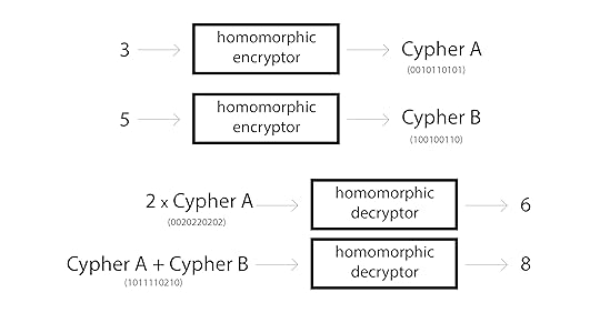
Now, there are a growing number of homomorphic encryption schemes, each with different properties. It's a relatively young field and there are several significant problems still being worked through, but we'll come back to that later.

For now, let's just start with the following. Integer public key encryption schemes that are homomorphic over multiplication and addition can perform the operations in the picture above. Furthermore, because the public key allows for "one way" encryption, you can even perform operations between unencrypted numbers and encrypted numbers (by one-way encrypting them), as exemplified above by 2 * Cypher A. (Some encryption schemes don't even require that... but again... we'll come back to that later)

Part 3: Can we use them together?

Perhaps the most frequent intersection between Deep Learning and Homomorphic Encryption has manifested around Data Privacy. As it turns out, when you homomorphically encrypt data, you can't read it but you still maintain most of the interesting statistical structure. This has allowed people to train models on encrypted data (CryptoNets). Furthermore a startup hedge fund called Numer.ai encrypts expensive, proprietary data and allows anyone to attempt to train machine learning models to predict the stock market. Normally they wouldn't be able to do this becuase it would constitute giving away incredibly expensive information. (and normal encryption would make model training impossible)

However, this blog post is about doing the inverse, encrypting the neural network and training it on decrypted data.

A neural network, in all its amazing complexity, actually breaks down into a surprisingly small number of moving parts which are simply repeated over and over again. In fact, many state-of-the-art neural networks can be created using only the following operations:

Addition
Multiplication
Division
Subtraction
Sigmoid
Tanh
Exponential

So, let's ask the obvious technical question, can we homomorphically encrypt the neural network itself? Would we want to? As it turns out, with a few conservative approximations, this can be done.

Addition - works out of the box
Multiplication - works out of the box
Division - works out of the box? - simply 1 / multiplication
Subtraction - works out of the box? - simply negated addition
Sigmoid - hmmm... perhaps a bit harder
Tanh - hmmm... perhaps a bit harder
Exponential - hmmm... perhaps a bit harder

It seems like we'll be able to get Division and Subtraction pretty trivially, but these more complicated functions are... well... more complicated than simple addition and multiplication. In order to try to homomorphically encrypt a deep neural network, we need one more secret ingredient.

Part 4: Taylor Series Expansion

Perhaps you remember it from primary school. A Taylor Series allows one to compute a complicated (nonlinear) function using an infinite series of additions, subtractions, multiplications, and divisions. This is perfect! (except for the infinite part). Fortunately, if you stop short of computing the exact Taylor Series Expansion you can still get a close approximation of the function at hand. Here are a few popular functions approximated via Taylor Series (Source).

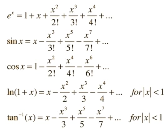
WAIT! THERE ARE EXPONENTS! No worries. Exponents are just repeated multiplication, which we can do. For something to play with, here's a little python implementation approximating the Taylor Series for our desirable sigmoid function (the formula for which you can lookup on Wolfram Alpha). We'll take the first few parts of the series and see how close we get to the true sigmoid function.

With only the first four factors of the Taylor Series, we get very close to sigmoid for a relatively large series of numbers. Now that we have our general strategy, it's time to select a Homomorphic Encryption algorithm.

Part 5: Choosing an Encryption Algorithm

Homomorphic Encryption is a relatively new field, with the major landmark being the discovery of the first Fully Homomorphic algorithm by Craig Gentry in 2009. This landmark event created a foothold for many to follow. Most of the excitement around Homomorphic Encryption has been around developing Turing Complete, homomorphically encrypted computers. Thus, the quest for a fully homomorphic scheme seeks to find an algorithm that can efficiently and securely compute the various logic gates required to run arbitrary computation. The general hope is that people would be able to securely offload work to the cloud with no risk that the data being sent could be read by anyone other than the sender. It's a very cool idea, and a lot of progress has been made.

However, there are some drawbacks. In general, most Fully Homomorphic Encryption schemes are incredibly slow relative to normal computers (not yet practical). This has sparked an interesting thread of research to limit the number of operations to be Somewhat homomorphic so that at least some computations could be performed. Less flexible but faster, a common tradeoff in computation.

This is where we want to start looking. In theory, we want a homomorphic encryption scheme that operates on floats (but we'll settle for integers, as we'll see) instead of binary values. Binary values would work, but not only would it require the flexibility of Fully Homomorphic Encryption (costing performance), but we'd have to manage the logic between binary representations and the math operations we want to compute. A less powerful, tailored HE algorithm for floating point operations would be a better fit.

Despite this constraint, there is still a plethora of choices. Here are a few popular ones with characterics we like:

Efficient Homomorphic Encryption on Integer Vectors and Its Applications
Yet Another Somewhat Homomorphic Encryption (YASHE)
Somewhat Practical Fully Homomorphic Encryption (FV)
Fully Homomorphic Encryption without Bootstrapping

The best one to use here is likely either YASHE or FV. YASHE was the method used for the popular CryptoNets algorithm, with great support for floating point operations. However, it's pretty complex. For the purpose of making this blogpost easy and fun to play around with, we're going to go with the slightly less advanced (and possibly less secure) Efficient Integer Vector Homomorphic Encryption. However, I think it's important to note that new HE algorithms are being developed as you read this, and the ideas presented in this blogpost are generic to any schemes that are homomorphic over addition and multiplication of integers and/or floating point numbers. If anything, it is my hope to raise awareness for this application of HE such that more HE algos will be developed to optimize for Deep Learning.

This encryption algorithm is also covered extensively by Yu, Lai, and Paylor in this work with an accompanying implementation here. The main bulk of the approach is in the C file vhe.cpp. Below we'll walk through a python port of this code with accompanying explanation for what's going on. This will also be useful if you choose to implement a more advanced scheme as there are themes that are relatively universal (general function names, variable names, etc.).

Part 6: Homomorphic Encryption in Python

Let���s start by covering a bit of the Homomorphic Encryption jargon:

Plaintext: this is your un-encrypted data. It's also called the "message". In our case, this will be a bunch of numbers representing our neural network.
Cyphertext: this is your encrypted data. We'll do math operations on the cyphertext which will change the underlying Plaintext.
Public Key: this is a pseudo-random sequence of numbers that allows anyone to encrypt data. It's ok to share this with people because (in theory) they can only use it for encryption.
Private/Secret Key: this is a pseudo-random sequence of numbers that allows you to decrypt data that was encrypted by the Public Key. You do NOT want to share this with people. Otherwise, they could decrypt your messages.

So, those are the major moving parts. They also correspond to particular variables with names that are pretty standard across different homomorphic encryption techniques. In this paper, they are the following:

S: this is a matrix that represents your Secret/Private Key. You need it to decrypt stuff.
M: This is your public key. You'll use it to encrypt stuff and perform math operations. Some algorithms don't require the public key for all math operations but this one uses it quite extensively.
c: This vector is your encrypted data, your "cyphertext".
x: This corresponds to your message, or your "plaintext". Some papers use the variable "m" instead.
w: This is a single "weighting" scalar variable which we use to re-weight our input message x (make it consistently bigger or smaller). We use this variable to help tune the signal/noise ratio. Making the signal "bigger" makes it less susceptible to noise at any given operation. However, making it too big increases our likelihood of corrupting our data entirely. It's a balance.
E or e: generally refers to random noise. In some cases, this refers to noise added to the data before encrypting it with the public key. This noise is generally what makes the decryption difficult. It's what allows two encryptions of the same message to be different, which is important to make the message hard to crack. Note, this can be a vector or a matrix depending on the algorithm and implementation. In other cases, this can refer to the noise that accumulates over operations. More on that later.

As is convention with many math papers, capital letters correspond to matrices, lowercase letters correspond to vectors, and italic lowercase letters correspond to scalars.

Homomorphic Encryption has four kinds of operations that we care about: public/private keypair generation, one-way encryption, decryption, and the math operations. Let's start with decryption.

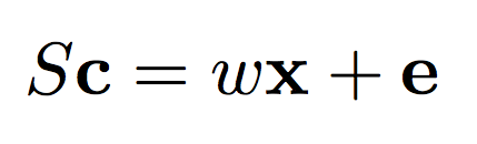
The formula on the left describes the general relationship between our secret key S and our message x. The formula on the right shows how we can use our secret key to decrypt our message. Notice that "e" is gone? Basically, the general philosophy of Homomorphic Encryption techniques is to introduce just enough noise that the original message is hard to get back without the secret key, but a small enough amount of noise that it amounts to a rounding error when you DO have the secret key. The brackets on the top and bottom represent "round to the nearest integer". Other Homomorphic Encryption algorithms round to various amounts. Modulus operators are nearly ubiquitous.

Encryption, then, is about generating a c so that this relationship holds true. If S is a random matrix, then c will be hard to decrypt. The simpler, non-symmetric way of generating an encryption key is to just find the inverse of the secret key. Let's start there with some Python code.

import numpy as np

def generate_key(w,m,n):
S = (np.random.rand(m,n) * w / (2 ** 16)) # proving max(S) < w
return S

def encrypt(x,S,m,n,w):
assert len(x) == len(S)

e = (np.random.rand(m)) # proving max(e) < w / 2
c = np.linalg.inv(S).dot((w * x) e)
return c

def decrypt(c,S,w):
return (S.dot(c) / w).astype('int')

def get_c_star(c,m,l):
c_star = np.zeros(l * m,dtype='int')
for i in range(m):
b = np.array(list(np.binary_repr(np.abs(c[i]))),dtype='int')
if(c[i] < 0):
b *= -1
c_star[(i * l) (l-len(b)): (i 1) * l] = b
return c_star

def get_S_star(S,m,n,l):
S_star = list()
for i in range(l):
S_star.append(S*2**(l-i-1))
S_star = np.array(S_star).transpose(1,2,0).reshape(m,n*l)
return S_star


x = np.array([0,1,2,5])

m = len(x)
n = m
w = 16
S = generate_key(w,m,n)

And when I run this code in an iPython notebook, I can perform the following operations (with corresponding output).

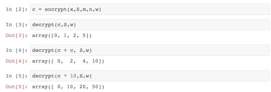
The key thing to look at are the bottom results. Notice that we can perform some basic operations to the cyphertext and it changes the underlying plaintext accordingly. Neat, eh?

Part 7: Optimizing Encryption

Import Lesson: Take a look at the decryption formulas again. If the secret key, S, is the identity matrix, then cyphertext c is just a re-weighted, slightly noisy version of the input x, which could easily be discovered given a handful of examples. If this doesn't make sense, Google "Identity Matrix Tutorial" and come back. It's a bit too much to go into here.

This leads us into how encryption takes place. Instead of explicitly allocating a self-standing "Public Key" and "Private Key", the authors propose a "Key Switching" technique, wherein they can swap out one Private Key S for another S'. More specifically, this private key switching technique involves generating a matrix M that can perform the transformation.Since M has the ability to convert a message from being unencrypted (secret key of the identity matrix) to being encrypted (secret key that's random and difficult to guess), this M becomes our public key!

That was a lot of information at a fast pace. Let's nutshell that again.

Here's what happened...


Given the two formulas above, if the secret key is the identity matrix, the message isn't encrypted.
Given the two formulas above, if the secret key is a random matrix, the generated message is encrypted.
We can make a matrix M that changes the secret key from one secret key to another.
When the matrix M converts from the identity to a random secret key, it is, by extension, encrypting the message in a one-way encryption.
Because M performs the role of a "one way encryption", we call it the "public key" and can distribute it like we would a public key since it cannot decrypt the code.


So, without further adue, let's see how this is done in Python.



import numpy as np

def generate_key(w,m,n):
S = (np.random.rand(m,n) * w / (2 ** 16)) # proving max(S) < w
return S

def encrypt(x,S,m,n,w):
assert len(x) == len(S)

e = (np.random.rand(m)) # proving max(e) < w / 2
c = np.linalg.inv(S).dot((w * x) e)
return c

def decrypt(c,S,w):
return (S.dot(c) / w).astype('int')

def get_c_star(c,m,l):
c_star = np.zeros(l * m,dtype='int')
for i in range(m):
b = np.array(list(np.binary_repr(np.abs(c[i]))),dtype='int')
if(c[i] < 0):
b *= -1
c_star[(i * l) (l-len(b)): (i 1) * l] = b
return c_star

def switch_key(c,S,m,n,T):
l = int(np.ceil(np.log2(np.max(np.abs(c)))))
c_star = get_c_star(c,m,l)
S_star = get_S_star(S,m,n,l)
n_prime = n 1


S_prime = np.concatenate((np.eye(m),T.T),0).T
A = (np.random.rand(n_prime - m, n*l) * 10).astype('int')
E = (1 * np.random.rand(S_star.shape[0],S_star.shape[1])).astype('int')
M = np.concatenate(((S_star - T.dot(A) E),A),0)
c_prime = M.dot(c_star)
return c_prime,S_prime

def get_S_star(S,m,n,l):
S_star = list()
for i in range(l):
S_star.append(S*2**(l-i-1))
S_star = np.array(S_star).transpose(1,2,0).reshape(m,n*l)
return S_star

def get_T(n):
n_prime = n 1
T = (10 * np.random.rand(n,n_prime - n)).astype('int')
return T

def encrypt_via_switch(x,w,m,n,T):
c,S = switch_key(x*w,np.eye(m),m,n,T)
return c,S

x = np.array([0,1,2,5])

m = len(x)
n = m
w = 16
S = generate_key(w,m,n)

The way this works is by making the S key mostly the identiy matrix, simply concatenating a random vector T onto it. Thus, T really has all the information necessary for the secret key, even though we have to still create a matrix of size S to get things to work right.

Part 8: Building an XOR Neural Network

So, now that we know how to encrypt and decrypt messages (And compute basic addition and multiplication), it's time to start trying to expand to the rest of the operations we need to build a simple XOR neural network. While technically neural networks are just a series of very simple operations, there are several combinations of these operations that we need some handy functions for. So, here I'm going to describe each operation we need and the high level approach we're going to take (basically which series of additions and multiplications we'll use). Then I'll show you code. For detailed descriptions check out this work


Floating Point Numbers: We're going to do this by simply scaling our floats into integers. We'll train our network on integers as if they were floats. Let's say we're scaling by 1000. 0.2 * 0.5 = 0.1. If we scale up, 200 * 500 = 100000. We have to scale down by 1000 twice since we performed multiplication, but 100000 / (1000 * 1000) = 0.1 which is what we want. This can be tricky at first but you'll get used to it. Since this HE scheme rounds to the nearest integer, this also lets you control the precision of your neural net.
Vector-Matrix Multiplication: This is our bread and butter. As it turns out, the M matrix that converts from one secret key to another is actually a way to linear transform.
Inner Dot Product: In the right context, the linear transformation above can also be an inner dot product.
Sigmoid: Since we can do vector-matrix multiplication, we can evaluate arbitrary polynomials given enough multiplications. Since we know the Taylor Series polynomial for sigmoid, we can evaluate an approximate sigmoid!
Elementwise Matrix Multiplication: This one is surprisingly inefficient. We have to do a Vector-Matrix multiplication or a series of inner dot products.
Outer Product: We can accomplish this via masking and inner products.




As a general disclaimer, there might be more effient ways of accomplishing these methods, but I didn't want to risk compromising the integrity of the homomorphic encryption scheme, so I sortof bent over backwards to just use the provided functions from the paper (with the allowed extension to sigmoid). Now, let's see how these are accomplished in Python.



def sigmoid(layer_2_c):
out_rows = list()
for position in range(len(layer_2_c)-1):

M_position = M_onehot[len(layer_2_c)-2][0]

layer_2_index_c = innerProd(layer_2_c,v_onehot[len(layer_2_c)-2][position],M_position,l) / scaling_factor

x = layer_2_index_c
x2 = innerProd(x,x,M_position,l) / scaling_factor
x3 = innerProd(x,x2,M_position,l) / scaling_factor
x5 = innerProd(x3,x2,M_position,l) / scaling_factor
x7 = innerProd(x5,x2,M_position,l) / scaling_factor

xs = copy.deepcopy(v_onehot[5][0])
xs[1] = x[0]
xs[2] = x2[0]
xs[3] = x3[0]
xs[4] = x5[0]
xs[5] = x7[0]

out = mat_mul_forward(xs,H_sigmoid[0:1],scaling_factor)
out_rows.append(out)
return transpose(out_rows)[0]

def load_linear_transformation(syn0_text,scaling_factor = 1000):
syn0_text *= scaling_factor
return linearTransformClient(syn0_text.T,getSecretKey(T_keys[len(syn0_text)-1]),T_keys[len(syn0_text)-1],l)

def outer_product(x,y):
flip = False
if(len(x) < len(y)):
flip = True
tmp = x
x = y
y = tmp

y_matrix = list()

for i in range(len(x)-1):
y_matrix.append(y)

y_matrix_transpose = transpose(y_matrix)

outer_result = list()
for i in range(len(x)-1):
outer_result.append(mat_mul_forward(x * onehot[len(x)-1][i],y_matrix_transpose,scaling_factor))

if(flip):
return transpose(outer_result)

return outer_result

def mat_mul_forward(layer_1,syn1,scaling_factor):

input_dim = len(layer_1)
output_dim = len(syn1)

buff = np.zeros(max(output_dim 1,input_dim 1))
buff[0:len(layer_1)] = layer_1
layer_1_c = buff

syn1_c = list()
for i in range(len(syn1)):
buff = np.zeros(max(output_dim 1,input_dim 1))
buff[0:len(syn1[i])] = syn1[i]
syn1_c.append(buff)

layer_2 = innerProd(syn1_c[0],layer_1_c,M_onehot[len(layer_1_c) - 2][0],l) / float(scaling_factor)
for i in range(len(syn1)-1):
layer_2 = innerProd(syn1_c[i 1],layer_1_c,M_onehot[len(layer_1_c) - 2][i 1],l) / float(scaling_factor)
return layer_2[0:output_dim 1]

def elementwise_vector_mult(x,y,scaling_factor):

y =[y]

one_minus_layer_1 = transpose(y)

outer_result = list()
for i in range(len(x)-1):
outer_result.append(mat_mul_forward(x * onehot[len(x)-1][i],y,scaling_factor))

return transpose(outer_result)[0]



Now, there's one bit that I haven't told you about yet. To save time, I'm pre-computing several keys, , vectors, and matrices and storing them. This includes things like "the vector of all 1s" and one-hot encoding vectors of various lengths. This is useful for the masking operations above as well as some simple things we want to be able to do. For example, the derivive of sigmoid is sigmoid(x) * (1 - sigmoid(x)). Thus, precomputing these variables is handy. Here's the pre-computation step.



# HAPPENS ON SECURE SERVER

l = 100
w = 2 ** 25

aBound = 10
tBound = 10
eBound = 10

max_dim = 10

scaling_factor = 1000

# keys
T_keys = list()
for i in range(max_dim):
T_keys.append(np.random.rand(i 1,1))

# one way encryption transformation
M_keys = list()
for i in range(max_dim):
M_keys.append(innerProdClient(T_keys[i],l))

M_onehot = list()
for h in range(max_dim):
i = h 1
buffered_eyes = list()
for row in np.eye(i 1):
buffer = np.ones(i 1)
buffer[0:i 1] = row
buffered_eyes.append((M_keys[i-1].T * buffer).T)
M_onehot.append(buffered_eyes)

c_ones = list()
for i in range(max_dim):
c_ones.append(encrypt(T_keys[i],np.ones(i 1), w, l).astype('int'))

v_onehot = list()
onehot = list()
for i in range(max_dim):
eyes = list()
eyes_txt = list()
for eye in np.eye(i 1):
eyes_txt.append(eye)
eyes.append(one_way_encrypt_vector(eye,scaling_factor))
v_onehot.append(eyes)
onehot.append(eyes_txt)

H_sigmoid_txt = np.zeros((5,5))

H_sigmoid_txt[0][0] = 0.5
H_sigmoid_txt[0][1] = 0.25
H_sigmoid_txt[0][2] = -1/48.0
H_sigmoid_txt[0][3] = 1/480.0
H_sigmoid_txt[0][4] = -17/80640.0

H_sigmoid = list()
for row in H_sigmoid_txt:
H_sigmoid.append(one_way_encrypt_vector(row))




If you're looking closely, you'll notice that the H_sigmoid matrix is the matrix we need for the polynomial evaluation of sigmoid. :) Finally, we want to train our neural network with the following. If the neural netowrk parts don't make sense, review A Neural Network in 11 Lines of Python. I've basically taken the XOR network from there and swapped out its operations with the proper utility functions for our encrypted weights.



np.random.seed(1234)

input_dataset = [[],[0],[1],[0,1]]
output_dataset = [[0],[1],[1],[0]]

input_dim = 3
hidden_dim = 4
output_dim = 1
alpha = 0.015

# one way encrypt our training data using the public key (this can be done onsite)
y = list()
for i in range(4):
y.append(one_way_encrypt_vector(output_dataset[i],scaling_factor))

# generate our weight values
syn0_t = (np.random.randn(input_dim,hidden_dim) * 0.2) - 0.1
syn1_t = (np.random.randn(output_dim,hidden_dim) * 0.2) - 0.1

# one-way encrypt our weight values
syn1 = list()
for row in syn1_t:
syn1.append(one_way_encrypt_vector(row,scaling_factor).astype('int64'))

syn0 = list()
for row in syn0_t:
syn0.append(one_way_encrypt_vector(row,scaling_factor).astype('int64'))


# begin training
for iter in range(1000):

decrypted_error = 0
encrypted_error = 0
for row_i in range(4):

if(row_i == 0):
layer_1 = sigmoid(syn0[0])
elif(row_i == 1):
layer_1 = sigmoid((syn0[0] syn0[1])/2.0)
elif(row_i == 2):
layer_1 = sigmoid((syn0[0] syn0[2])/2.0)
else:
layer_1 = sigmoid((syn0[0] syn0[1] syn0[2])/3.0)

layer_2 = (innerProd(syn1[0],layer_1,M_onehot[len(layer_1) - 2][0],l) / float(scaling_factor))[0:2]

layer_2_delta = add_vectors(layer_2,-y[row_i])

syn1_trans = transpose(syn1)

one_minus_layer_1 = [(scaling_factor * c_ones[len(layer_1) - 2]) - layer_1]
sigmoid_delta = elementwise_vector_mult(layer_1,one_minus_layer_1[0],scaling_factor)
layer_1_delta_nosig = mat_mul_forward(layer_2_delta,syn1_trans,1).astype('int64')
layer_1_delta = elementwise_vector_mult(layer_1_delta_nosig,sigmoid_delta,scaling_factor) * alpha

syn1_delta = np.array(outer_product(layer_2_delta,layer_1)).astype('int64')

syn1[0] -= np.array(syn1_delta[0]* alpha).astype('int64')

syn0[0] -= (layer_1_delta).astype('int64')

if(row_i == 1):
syn0[1] -= (layer_1_delta).astype('int64')
elif(row_i == 2):
syn0[2] -= (layer_1_delta).astype('int64')
elif(row_i == 3):
syn0[1] -= (layer_1_delta).astype('int64')
syn0[2] -= (layer_1_delta).astype('int64')


# So that we can watch training, I'm going to decrypt the loss as we go.
# If this was a secure environment, I wouldn't be doing this here. I'd send
# the encrypted loss somewhere else to be decrypted
encrypted_error = int(np.sum(np.abs(layer_2_delta)) / scaling_factor)
decrypted_error = np.sum(np.abs(s_decrypt(layer_2_delta).astype('float')/scaling_factor))


sys.stdout.write("\r Iter:" str(iter) " Encrypted Loss:" str(encrypted_error) " Decrypted Loss:" str(decrypted_error) " Alpha:" str(alpha))

# just to make logging nice
if(iter % 10 == 0):
print()

# stop training when encrypted error reaches a certain level
if(encrypted_error < 25000000):
break

print("\nFinal Prediction:")

for row_i in range(4):

if(row_i == 0):
layer_1 = sigmoid(syn0[0])
elif(row_i == 1):
layer_1 = sigmoid((syn0[0] syn0[1])/2.0)
elif(row_i == 2):
layer_1 = sigmoid((syn0[0] syn0[2])/2.0)
else:
layer_1 = sigmoid((syn0[0] syn0[1] syn0[2])/3.0)

layer_2 = (innerProd(syn1[0],layer_1,M_onehot[len(layer_1) - 2][0],l) / float(scaling_factor))[0:2]
print("True Pred:" str(output_dataset[row_i]) " Encrypted Prediction:" str(layer_2) " Decrypted Prediction:" str(s_decrypt(layer_2) / scaling_factor))





Iter:0 Encrypted Loss:84890656 Decrypted Loss:2.529 Alpha:0.015
Iter:10 Encrypted Loss:69494197 Decrypted Loss:2.071 Alpha:0.015
Iter:20 Encrypted Loss:64017850 Decrypted Loss:1.907 Alpha:0.015
Iter:30 Encrypted Loss:62367015 Decrypted Loss:1.858 Alpha:0.015
Iter:40 Encrypted Loss:61874493 Decrypted Loss:1.843 Alpha:0.015
Iter:50 Encrypted Loss:61399244 Decrypted Loss:1.829 Alpha:0.015
Iter:60 Encrypted Loss:60788581 Decrypted Loss:1.811 Alpha:0.015
Iter:70 Encrypted Loss:60327357 Decrypted Loss:1.797 Alpha:0.015
Iter:80 Encrypted Loss:59939426 Decrypted Loss:1.786 Alpha:0.015
Iter:90 Encrypted Loss:59628769 Decrypted Loss:1.778 Alpha:0.015
Iter:100 Encrypted Loss:59373621 Decrypted Loss:1.769 Alpha:0.015
Iter:110 Encrypted Loss:59148014 Decrypted Loss:1.763 Alpha:0.015
Iter:120 Encrypted Loss:58934571 Decrypted Loss:1.757 Alpha:0.015
Iter:130 Encrypted Loss:58724873 Decrypted Loss:1.75 Alpha:0.0155
Iter:140 Encrypted Loss:58516008 Decrypted Loss:1.744 Alpha:0.015
Iter:150 Encrypted Loss:58307663 Decrypted Loss:1.739 Alpha:0.015
Iter:160 Encrypted Loss:58102049 Decrypted Loss:1.732 Alpha:0.015
Iter:170 Encrypted Loss:57863091 Decrypted Loss:1.725 Alpha:0.015
Iter:180 Encrypted Loss:55470158 Decrypted Loss:1.653 Alpha:0.015
Iter:190 Encrypted Loss:54650383 Decrypted Loss:1.629 Alpha:0.015
Iter:200 Encrypted Loss:53838756 Decrypted Loss:1.605 Alpha:0.015
Iter:210 Encrypted Loss:51684722 Decrypted Loss:1.541 Alpha:0.015
Iter:220 Encrypted Loss:54408709 Decrypted Loss:1.621 Alpha:0.015
Iter:230 Encrypted Loss:54946198 Decrypted Loss:1.638 Alpha:0.015
Iter:240 Encrypted Loss:54668472 Decrypted Loss:1.63 Alpha:0.0155
Iter:250 Encrypted Loss:55444008 Decrypted Loss:1.653 Alpha:0.015
Iter:260 Encrypted Loss:54094286 Decrypted Loss:1.612 Alpha:0.015
Iter:270 Encrypted Loss:51251831 Decrypted Loss:1.528 Alpha:0.015
Iter:276 Encrypted Loss:24543890 Decrypted Loss:0.732 Alpha:0.015
Final Prediction:
True Pred:[0] Encrypted Prediction:[-3761423723.0718255 0.0] Decrypted Prediction:[-0.112]
True Pred:[1] Encrypted Prediction:[24204806753.166267 0.0] Decrypted Prediction:[ 0.721]
True Pred:[1] Encrypted Prediction:[23090462896.17028 0.0] Decrypted Prediction:[ 0.688]
True Pred:[0] Encrypted Prediction:[1748380342.4553354 0.0] Decrypted Prediction:[ 0.052]



When I train this neural network, this is the output that I see. Tuning was a bit tricky as some combination of the encryption noise and the low precision creates for somewhat chunky learning. Training is also quite slow. A lot of this comes back to how expensive the transpose operation is. I'm pretty sure that I could do something quite a bit simpler, but, again, I wanted to air on the side of safety for this proof of concept.




Things to takeaway:



The weights of the network are all encrypted.
The data is decrypted... 1s and 0s.
After training, the network could be decrypted for increased performance or training (or switch to a different encryption key).
The training loss and output predictions are all also encrypted values. We have to decode them in order to be able to interpret the network.



Part 9: Sentiment Classification

To make this a bit more real, here's the same network training on IMDB sentiment reviews based on a network from Udacity's Deep Learning Nanodegree. You can find the full code here



import time
import sys
import numpy as np

# Let's tweak our network from before to model these phenomena
class SentimentNetwork:
def __init__(self, reviews,labels,min_count = 10,polarity_cutoff = 0.1,hidden_nodes = 8, learning_rate = 0.1):

np.random.seed(1234)

self.pre_process_data(reviews, polarity_cutoff, min_count)

self.init_network(len(self.review_vocab),hidden_nodes, 1, learning_rate)


def pre_process_data(self,reviews, polarity_cutoff,min_count):

print("Pre-processing data...")

positive_counts = Counter()
negative_counts = Counter()
total_counts = Counter()

for i in range(len(reviews)):
if(labels[i] == 'POSITIVE'):
for word in reviews[i].split(" "):
positive_counts[word] = 1
total_counts[word] = 1
else:
for word in reviews[i].split(" "):
negative_counts[word] = 1
total_counts[word] = 1

pos_neg_ratios = Counter()

for term,cnt in list(total_counts.most_common()):
if(cnt >= 50):
pos_neg_ratio = positive_counts[term] / float(negative_counts[term] 1)
pos_neg_ratios[term] = pos_neg_ratio

for word,ratio in pos_neg_ratios.most_common():
if(ratio > 1):
pos_neg_ratios[word] = np.log(ratio)
else:
pos_neg_ratios[word] = -np.log((1 / (ratio 0.01)))

review_vocab = set()
for review in reviews:
for word in review.split(" "):
if(total_counts[word] > min_count):
if(word in pos_neg_ratios.keys()):
if((pos_neg_ratios[word] >= polarity_cutoff) or (pos_neg_ratios[word] <= -polarity_cutoff)):
review_vocab.add(word)
else:
review_vocab.add(word)
self.review_vocab = list(review_vocab)

label_vocab = set()
for label in labels:
label_vocab.add(label)

self.label_vocab = list(label_vocab)

self.review_vocab_size = len(self.review_vocab)
self.label_vocab_size = len(self.label_vocab)

self.word2index = {}
for i, word in enumerate(self.review_vocab):
self.word2index[word] = i

self.label2index = {}
for i, label in enumerate(self.label_vocab):
self.label2index[label] = i


def init_network(self, input_nodes, hidden_nodes, output_nodes, learning_rate):
# Set number of nodes in input, hidden and output layers.
self.input_nodes = input_nodes
self.hidden_nodes = hidden_nodes
self.output_nodes = output_nodes

print("Initializing Weights...")
self.weights_0_1_t = np.zeros((self.input_nodes,self.hidden_nodes))

self.weights_1_2_t = np.random.normal(0.0, self.output_nodes**-0.5,
(self.hidden_nodes, self.output_nodes))

print("Encrypting Weights...")
self.weights_0_1 = list()
for i,row in enumerate(self.weights_0_1_t):
sys.stdout.write("\rEncrypting Weights from Layer 0 to Layer 1:" str(float((i 1) * 100) / len(self.weights_0_1_t))[0:4] "% done")
self.weights_0_1.append(one_way_encrypt_vector(row,scaling_factor).astype('int64'))
print("")

self.weights_1_2 = list()
for i,row in enumerate(self.weights_1_2_t):
sys.stdout.write("\rEncrypting Weights from Layer 1 to Layer 2:" str(float((i 1) * 100) / len(self.weights_1_2_t))[0:4] "% done")
self.weights_1_2.append(one_way_encrypt_vector(row,scaling_factor).astype('int64'))
self.weights_1_2 = transpose(self.weights_1_2)

self.learning_rate = learning_rate

self.layer_0 = np.zeros((1,input_nodes))
self.layer_1 = np.zeros((1,hidden_nodes))

def sigmoid(self,x):
return 1 / (1 np.exp(-x))


def sigmoid_output_2_derivative(self,output):
return output * (1 - output)

def update_input_layer(self,review):

# clear out previous state, reset the layer to be all 0s
self.layer_0 *= 0
for word in review.split(" "):
self.layer_0[0][self.word2index[word]] = 1

def get_target_for_label(self,label):
if(label == 'POSITIVE'):
return 1
else:
return 0

def train(self, training_reviews_raw, training_labels):

training_reviews = list()
for review in training_reviews_raw:
indices = set()
for word in review.split(" "):
if(word in self.word2index.keys()):
indices.add(self.word2index[word])
training_reviews.append(list(indices))

layer_1 = np.zeros_like(self.weights_0_1[0])

start = time.time()
correct_so_far = 0
total_pred = 0.5
for i in range(len(training_reviews_raw)):
review_indices = training_reviews[i]
label = training_labels[i]

layer_1 *= 0
for index in review_indices:
layer_1 = self.weights_0_1[index]
layer_1 = layer_1 / float(len(review_indices))
layer_1 = layer_1.astype('int64') # round to nearest integer

layer_2 = sigmoid(innerProd(layer_1,self.weights_1_2[0],M_onehot[len(layer_1) - 2][1],l) / float(scaling_factor))[0:2]

if(label == 'POSITIVE'):
layer_2_delta = layer_2 - (c_ones[len(layer_2) - 2] * scaling_factor)
else:
layer_2_delta = layer_2

weights_1_2_trans = transpose(self.weights_1_2)
layer_1_delta = mat_mul_forward(layer_2_delta,weights_1_2_trans,scaling_factor).astype('int64')

self.weights_1_2 -= np.array(outer_product(layer_2_delta,layer_1)) * self.learning_rate

for index in review_indices:
self.weights_0_1[index] -= (layer_1_delta * self.learning_rate).astype('int64')

# we're going to decrypt on the fly so we can watch what's happening
total_pred = (s_decrypt(layer_2)[0] / scaling_factor)
if((s_decrypt(layer_2)[0] / scaling_factor) >= (total_pred / float(i 2)) and label == 'POSITIVE'):
correct_so_far = 1
if((s_decrypt(layer_2)[0] / scaling_factor) < (total_pred / float(i 2)) and label == 'NEGATIVE'):
correct_so_far = 1

reviews_per_second = i / float(time.time() - start)

sys.stdout.write("\rProgress:" str(100 * i/float(len(training_reviews_raw)))[:4] "% Speed(reviews/sec):" str(reviews_per_second)[0:5] " #Correct:" str(correct_so_far) " #Trained:" str(i 1) " Training Accuracy:" str(correct_so_far * 100 / float(i 1))[:4] "%")
if(i % 100 == 0):
print(i)


def test(self, testing_reviews, testing_labels):

correct = 0

start = time.time()

for i in range(len(testing_reviews)):
pred = self.run(testing_reviews[i])
if(pred == testing_labels[i]):
correct = 1

reviews_per_second = i / float(time.time() - start)

sys.stdout.write("\rProgress:" str(100 * i/float(len(testing_reviews)))[:4] \
"% Speed(reviews/sec):" str(reviews_per_second)[0:5] \
"% #Correct:" str(correct) " #Tested:" str(i 1) " Testing Accuracy:" str(correct * 100 / float(i 1))[:4] "%")

def run(self, review):

# Input Layer


# Hidden layer
self.layer_1 *= 0
unique_indices = set()
for word in review.lower().split(" "):
if word in self.word2index.keys():
unique_indices.add(self.word2index[word])
for index in unique_indices:
self.layer_1 = self.weights_0_1[index]

# Output layer
layer_2 = self.sigmoid(self.layer_1.dot(self.weights_1_2))

if(layer_2[0] >= 0.5):
return "POSITIVE"
else:
return "NEGATIVE"





Progress:0.0% Speed(reviews/sec):0.0 #Correct:1 #Trained:1 Training Accuracy:100.%0
Progress:0.41% Speed(reviews/sec):1.978 #Correct:66 #Trained:101 Training Accuracy:65.30
Progress:0.83% Speed(reviews/sec):2.014 #Correct:131 #Trained:201 Training Accuracy:65.1 0
Progress:1.25% Speed(reviews/sec):2.011 #Correct:203 #Trained:301 Training Accuracy:67.400
Progress:1.66% Speed(reviews/sec):2.003 #Correct:276 #Trained:401 Training Accuracy:68.8@0
Progress:2.08% Speed(reviews/sec):2.007 #Correct:348 #Trained:501 Training Accuracy:69.4P0
Progress:2.5% Speed(reviews/sec):2.015 #Correct:420 #Trained:601 Training Accuracy:69.8`0
Progress:2.91% Speed(reviews/sec):1.974 #Correct:497 #Trained:701 Training Accuracy:70.8p0
Progress:3.33% Speed(reviews/sec):1.973 #Correct:581 #Trained:801 Training Accuracy:72.50
Progress:3.75% Speed(reviews/sec):1.976 #Correct:666 #Trained:901 Training Accuracy:73.90
Progress:4.16% Speed(reviews/sec):1.983 #Correct:751 #Trained:1001 Training Accuracy:75.000
Progress:4.33% Speed(reviews/sec):1.940 #Correct:788 #Trained:1042 Training Accuracy:75.6%
....


Part 10: Advantages over Data Encryption

The most similar approach to this one is to encrypt training data and train neural networks on the encrypted data (accepting encrypted input and predicting encrypted output). This is a fantastic idea. However, it does have a few drawbacks. First and foremost, encrypting the data means that the neural network is completely useless to anyone without the private key for the encrypted data. This makes it impossible for data from different private sources to be trained on the same Deep Learning model. Most commercial applications have this requirement, requiring the aggregation of consumer data. In theory, we'd want every consumer to be protected by their own secret key, but homomorphically encrypting the data requires that everyone use the SAME key.

However, encrypting the network doesn't have this restriction.

With the approach above, you could train a regular, decrypted neural network for a while, encrypt it, send it to Party A with a public key (who trains it for a while on their own data... which remains in their possession). Then, you could get the network back, decrypt it, re-encrypt it with a different key and send it to Party B who does some training on their data. Since the network itself is what's enrypted, you get total control over the intelligence that you're capturing along the way. Party A and Party B would have no way of knowing that they each received the same network, and this all happens without them ever being able to see or use the network on their own data. You, the company, retain control over the IP in the neural network, and each user retains control over their own data.

Part 11: Future Work

There are faster and more secure homomorphic encryption algorithms. Taking this work and porting it to YASHE is, I believe, a step in the right direction. Perhaps a frameowrk would be appropriate to make encryption easier for the user, as it has a few systemic complications. In general, in order for many of these ideas to reach production level quality, HE needs to get faster. However, progress is happening quickly. I'm sure we'll be there before too long.

Part 12: Potential Applications

Decentralized AI: Companies can deploy models to be trained or used in the field without risking their intelligence being stolen.

Protected Consumer Privacy: the previous application opens up the possibility that consumers could simply hold onto their data, and "opt in" to different models being trained on their lives, instead of sending their data somewhere else. Companies have less of an excuse if their IP isn't at risk via decentralization. Data is power and it needs to go back to the people.

Controlled Superintelligence: The network can become as smart as it wants, but unless it has the secret key, all it can do is predict jibberish.

EDIT: A complete revamp of PyTorch was released today (Jan 18, 2017), making this blogpost a bit obselete. I will update this post with a new Quickstart Guide soon, but for now you should check out their documentation.</a>

This Blogpost Will Cover:

Part 1: PyTorch Installation
Part 2: Matrices and Linear Algebra in PyTorch
Part 3: Building a Feedforward Network (starting with a familiar one )
Part 4: The State of PyTorch

Pre-Requisite Knowledge:

Simple Feedforward Neural Networks ( Tutorial )
Basic Gradient Descent ( Tutorial )

Torch is one of the most popular Deep Learning frameworks in the world, dominating much of the research community for the past few years (only recently being rivaled by major Google sponsored frameworks Tensorflow and Keras). Perhaps its only drawback to new users has been the fact that it requires one to know Lua, a language that used to be very uncommon in the Machine Learning community. Even today, this barrier to entry can seem a bit much for many new to the field, who are already in the midst of learning a tremendous amount, much less a completely new programming language.

However, thanks to the wonderful and billiant Hugh Perkins, Torch recently got a new face, PyTorch... and it's much more accessible to the python hacker turned Deep Learning Extraordinare than it's Luariffic cousin. I have a passion for tools that make Deep Learning accessible, and so I'd like to lay out a short "Unofficial Startup Guide" for those of you interested in taking it for a spin. Before we get started, however, a question:

Why Use a Framework like PyTorch? In the past, I have advocated learning Deep Learning using only a matrix library. For the purposes of actually knowing what goes on under the hood, I think that this is essential, and the lessons learned from building things from scratch are real gamechangers when it comes to the messiness of tackling real world problems with these tools. However, when building neural networks in the wild (Kaggle Competitions, Production Systems, and Research Experiments), it's best to use a framework.

Why? Frameworks such as PyTorch allow you (the researcher) to focus exclusively on your experiment and iterate very quickly. Want to swap out a layer? Most frameworks will let you do this with a single line code change. Want to run on a GPU? Many frameworks will take care of it (sometimes with 0 code changes). If you built the network by hand in a matrix library, you might be spending a few hours working out these kinds of modifications. So, for learning, use a linear algebra library (like Numpy). For applying, use a framework (like PyTorch). Let's get started!

For New Readers: I typically tweet out new blogposts when they're complete @iamtrask. Feel free to follow if you'd be interested in reading more in the future and thanks for all the upvotes on Hacker News and Reddit! They mean a lot to me.

Part 1: Installation

Install Torch: The first thing you need to do is install torch and the "nn" package using luarocks. As torch is a very robust framework, the installation instructions should work well for you. After that, you should be able to run:

luarocks install nn

and be good to go. If any of these steps fails to work, copy paste what looks like the "error" and error description (should just be one sentence or so) from the command line and put it into Google (as is common practice when installing).

Clone the Repository: At the time of writing, PyTorch doesn't seem to be in the PyPI repository. So, we'll need to clone the repo in order to install it. Assuming you have git already installed (hint hint... if not go install it and come back), you should open up your Terminal application and navigate to an empty folder. Personally, I have a folder called "Laboratory" in my home directory (i.e. "cd ~/Laboratory/"), which cators to various childhood memories of mine. If you're not sure where to put it, feel free to use your Desktop for now. Once there, execute the commands:

git clone https://github.com/hughperkins/pytorc...

cd pytorch/

pip install -r requirements.txt

pip install -r test/requirements.txt

source ~/torch/install/bin/torch-activate

./build.sh

For me, this worked flawlessly, finishing with the statement

Finished processing dependencies for PyTorch===4.1.1-SNAPSHOT

If you also see this output at the bottom of your terminal, congraulations! You have successfully installed PyTorch!

Startup Jupyter Notebook: While certainly not a requirement, I highly recommend playing around with this new tool using Jupyter Notebok, which is definitely best installed using conda. Take my word for it. Install it using conda. All other ways are madness.

Part 2: Matrices and Linear Algebra

In the spirit of starting with the basics, neural networks run on linear algebra libraries. PyTorch is no exception. So, the simplest building block of PyTorch is its linear algebra library.

Above, I created 4 matrices. Notice that the library doesn't call them matrices though. It calls them tensors.

Quick Primer on Tensors: A Tensor is just a more generic term than matrix or vector. 1-dimensional tensors are vectors. 2-dimensional tensors are matrices. 3+ dimensional tensors are just refered to as tensors. If you're unfamiliar with these objects, here's a quick summary. A vector is "a list of numbers". A matrix is "a list of lists of numbers". A 3-d tensor is "a list of lists of lists of numbers". A 4-d tensor is... See the pattern? For more on how vectors and matrices are used to make neural networks, see my first blog post on a Neural Network in 11 lines of Python

PyTorch Tensors There appear to be 4 major types of tensors in PyTorch: Byte, Float, Double, and Long tensors. Each tensor type corresponds to the type of number (and more importantly the size/preision of the number) contained in each place of the matrix. So, if a 1-d Tensor is a "list of numbers", a 1-d Float Tensor is a list of floats. As a general rule of thumb, for weight matries we use FloatTensors. For data matrices, we'll likely use either FloatTensors (for real valued inputs) or Long Tensors (for integers). I'm a little bit surprised to not see IntTensor anywhere. Perhaps it has yet to be wrapped or is just non-obvious in the API.

The final thing to notice is that the matries seem to come with lots of rather random looking numbers inside (but not sensibly random like "evenly random between 0 and 1"). This is actually a plus of the library in my book. Let me explain (skip 1 paragraph if you're familiar with this concept)

Why Seemingly Nonsenical Values: When you create a new matrix in PyTorch, the framework goes and "sets aside" enough RAM memory to store your matrix. However, "setting aside" memory is completely different from "changing all the values in that memory to 0". "Setting aside" memory while also "changing all the values to 0" is more computationally expensive. It's nice that this library doesn't assume you want the values to be any particular way. Instead, it just sets aside memory and whatever 1s and 0s happen to be there from the last program that used that piece of RAM will show up in your matrix. In most cases, we're going to set the values in our matrices to be something else anyway (say... our input data values or a specific kind of random number range). So, the fact that it doesn't pre-set the matrix values saves you a bit of processing time, but the user needs to recognize that it's their responsibility to actively choose the values he/she wants in a matrix. Numpy is not like this, which make Numpy a bit more user friendly but also less computationally efficient.

Basic Linear Algebra Operations: So, now that we know how to store numbers in PyTorch, lets talk a bit about how PyTorch manipulates them. How does one go about doing linear algebra in PyTorch?

The Basic Neural Network Operations: Neural networks, amidst all their complexity, are actually mostly made up of rather simple operations. If you remember from A Neural Network in 11 Lines of Python, we can build a working network with only Matrix-Matrix Multiplication, Vector-Matrix Multiplication, Elementwise Operations (addition, subtraction, multiplication, and division), Matrix Transposition, and a handful of elementwise functions (sigmoid, and a special function to compute sigmoid's derivative at a point which uses only the aforementioned elementwise operations). Let's initialize some matrices and start with the elementwise operations.

Elementwise Operations: Above I have given several examples of elementwise addition. (simply replacing the "+" sign with - * or / will give you the others). These act mostly how you would expect them to act. A few hiccups here and there. Notably, if you accidentally add two Tensors that aren't aligned correctly (have different dimensions) the python kernel crashes as opposed to throwing an error. It could be just my machine, but error handling in wrappers is notoriously time consuming to finish. I expect this functionality will be worked out soon enough, and as we will see, there's a suitable substitute.

Vector/Matrix Multiplication: It appears that the native matrix multiplication functionality of Torch isn't wrapped. Instead, we get to use something a bit more familiar. (This feature is really, really cool.) Much of PyTorch can run on native numpy matrices. That's right! The convenient functionality of numpy is now integrated with one of the most popular Deep Learning Frameworks out there. So, how should you really do elementwise and matrix multipliplication? Just use numpy! For completeness sake, here's the same elementwise operations using PyTorch's numpy connector.

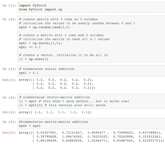
And now let's see how to do the basic matrix operations we need for a feedforward network.

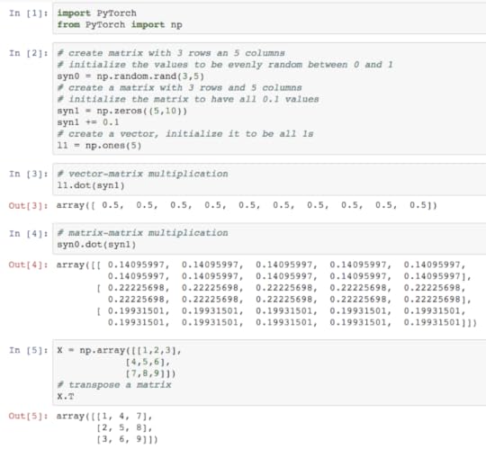
Other Neural Functions: Finally, we also need to be able to compute some nonlinearities efficiently. There are both numpy and native wrappers made available which seem to run quite fast. Additionally, sigmoid has a native implementation (something that numpy does not implement), which is quite nice and a bit faster than computing it explicitly in numpy.

I consider the fantastic integration between numpy and PyTorch to be one of the great selling points of this framework. I personally love prototyping with the full control of a matrix library, and PyTorch really respects this preference as an option. This is so nice relative to most other frameworks out there. +1 for PyTorch.

Part 3: Building a Feedforward Network

In this section, we really get to start seeing PyTorch shine. While understanding how matrices are handled is an important pre-requisite to learning a framework, the various layers of abstraction are where frameworks really become useful. In this section, we're going to take the bare bones 3 layer neural network from a previous blogpost and convert it to a network using PyTorch's neural network abstractions. In this way, as we wrap each part of the network with a piece of framework functionality, you'll know exactly what PyTorch is doing under the hood. Your goal in this section should be to relate the PyTorch abstractions (objects, function calls, etc.) in the PyTorch network we will build with the matrix operations in the numpy neural network (pictured below)s.

import PyTorch
from PyTorch import np

def nonlin(x,deriv=False):
if(deriv==True):
return x*(1-x)

return 1/(1+np.exp(-x))

X = np.array([[0,0,1],
[0,1,1],
[1,0,1],
[1,1,1]])

y = np.array([[0],
[1],
[1],
[0]])

np.random.seed(1)

# randomly initialize our weights with mean 0
syn0 = 2*np.random.random((3,4)) - 1
syn1 = 2*np.random.random((4,1)) - 1

for j in range(60000):

# Feed forward through layers 0, 1, and 2
l0 = X
l1 = nonlin(np.dot(l0,syn0))
l2 = nonlin(np.dot(l1,syn1))

# how much did we miss the target value?
l2_error = y - l2

if (j% 10000) == 0:
print("Error:" + str(np.mean(np.abs(l2_error))))

# in what direction is the target value?
# were we really sure? if so, don't change too much.
l2_delta = l2_error*nonlin(l2,deriv=True)

# how much did each l1 value contribute to the l2 error (according to the weights)?
l1_error = l2_delta.dot(syn1.T)

# in what direction is the target l1?
# were we really sure? if so, don't change too much.
l1_delta = l1_error * nonlin(l1,deriv=True)

# lets update our weights
syn1 += l1.T.dot(l2_delta)
syn0 += l0.T.dot(l1_delta)





Error:0.496410031903
Error:0.00858452565325
Error:0.00578945986251
Error:0.00462917677677
Error:0.00395876528027
Error:0.00351012256786

Now that we've seen how to build this network (more or less "by hand"), let's starting building the same network using PyTorch instead of numpy.

import PyTorch
from PyTorchAug import nn
from PyTorch import np

First, we want to import several packages from PyTorch. np is the numpy wrapper mentioned before. nn is the Neural Network package, which contains things like layer types, error measures, and network containers, as we'll see in a second.

# randomly initialize our weights with mean 0
net = nn.Sequential()
net.add(nn.Linear(3, 4))
net.add(nn.Sigmoid())
net.add(nn.Linear(4, 1))
net.add(nn.Sigmoid())
net.float()

The next section highlights the primary advantage of deep learning frameworks in general. Instead of declaring a bunch of weight matrices (like with numpy), we create layers and "glue" them together using nn.Sequential(). Contained in these "layer" objects is logic about how the layers are constructed, how each layer forward propagates predictions, and how each layer backpropagates gradients. nn.Sequential() knows how to combine these layers together to allow them to learn together when presented with a dataset, which is what we'll do next.

X = np.array([[0,0,1],
[0,1,1],
[1,0,1],
[1,1,1]]).astype('float32')

y = np.array([[0],
[1],
[1],
[0]]).astype('float32')

This section is largely the same as before. We create our input (X) and output (y) datasets as numpy matrices. PyTorch seemed to want these matrices to be float32 values in order to do the implicit cast from numpy to PyTorch tensor objects well, so I added an .astype('float32') to ensure they were the right type.

crit = nn.MSECriterion()
crit.float()

This one might look a little strange if you're not familiar with neural network error measures. As it turns out, you can measure "how much you missed" in a variety of different ways. How you measure error changes how a network prioritizes different errors when training (what kinds of errors should it take most seriously). In this case, we're going to use the "Mean Squared Error". For a more in-depth coverage of this, please see Chapter 4 of Grokking Deep Learning.




for j in range(2400):

net.zeroGradParameters()

# Feed forward through layers 0, 1, and 2
output = net.forward(X)

# how much did we miss the target value?
loss = crit.forward(output, y)
gradOutput = crit.backward(output, y)

# how much did each l1 value contribute to the l2 error (according to the weights)?
# in what direction is the target l1?
# were we really sure? if so, don't change too much.
gradInput = net.backward(X, gradOutput)

# lets update our weights
net.updateParameters(1)

if (j% 200) == 0:
print("Error:" + str(loss))

And now for the training of the network. I have annotated each section of the code with near identical annotations as the numpy network. In this way, if you look at them side by side, you should be able to see where each operation in the numpy network occurs in the PyTorch network.

One part might not look familiar. The "net.zeroGradParameters()" basically just zeros out all our "delta" matrices before a new iteration. In our numpy network, this was the l2_delta variable and l1_delta variable. PyTorch re-uses the same memory allocations each time you forward propgate / back propagate (to be efficient, similar to what was mentioned in the Matrices section), so in order to keep from accidentally re-using the gradients from the prevoius iteration, you need to re-set them to 0. This is also a standard practice for most popular deep learning frameworks.

Finally, Torch also separates your "loss" from your "gradient". In our (somewhat oversimplified) numpy network, we just computed an "error" measure. As it turns out, your pure "error" and "delta" are actually slightly different measures. (delta is the derivative of the error). Again, for deeper coverage, see Chatper 4 of GDL.

Putting it all together

import PyTorch
from PyTorchAug import nn
from PyTorch import np

# randomly initialize our weights with mean 0
net = nn.Sequential()
net.add(nn.Linear(3, 4))
net.add(nn.Sigmoid())
net.add(nn.Linear(4, 1))
net.add(nn.Sigmoid())
net.float()

X = np.array([[0,0,1],
[0,1,1],
[1,0,1],
[1,1,1]]).astype('float32')

y = np.array([[0],
[1],
[1],
[0]]).astype('float32')

crit = nn.MSECriterion()
crit.float()

for j in range(2400):

net.zeroGradParameters()

# Feed forward through layers 0, 1, and 2
output = net.forward(X)

# how much did we miss the target value?
loss = crit.forward(output, y)
gradOutput = crit.backward(output, y)

# how much did each l1 value contribute to the l2 error (according to the weights)?
# in what direction is the target l1?
# were we really sure? if so, don't change too much.
gradInput = net.backward(X, gradOutput)

# lets update our weights
net.updateParameters(1)

if (j% 200) == 0:
print("Error:" + str(loss))



Error:0.2521711587905884
Error:0.2500123083591461
Error:0.249952495098114
Error:0.24984735250473022
Error:0.2495250701904297
Error:0.2475520819425583
Error:0.22693687677383423
Error:0.13267411291599274
Error:0.04083901643753052
Error:0.016316475346684456
Error:0.008736669085919857
Error:0.005575092509388924

Your results may vary a bit. I do not yet see how random numbers are to be seeded. If I come across that in the future, I'll add an edit.

Part 4: The State of PyTorch

While still a new framework with lots of ground to cover to close the gap with its competitors, PyTorch already has a lot to offer. It looks like there's an LSTM test case in the works, and strong promise for building custom layers in .lua files that you can import into Python with some simple wrapper functions. If you want to build feedforward neural networks using the industry standard Torch backend without having to deal with Lua, PyTorch is what you're looking for. If you want to build custom layers or do some heavy sequence2sequence models, I think the framework will be there very soon (with documentation / test cases to describe best practices). Overall, I'm very excited to see where this framework goes, and I encourage you to Star/Follow it on Github

For New Readers: I typically tweet out new blogposts when they're complete at @iamtrask. Feel free to follow if you'd be interested in reading more in the future and thanks for all the upvotes on hacker news and reddit!

If you passed high school math and can hack around in Python, I want to teach you Deep Learning.

Edit: 50% Coupon Code: "mltrask" (expires August 26)

I've decided to write a Deep Learning book in the same style as my blog, teaching Deep Learning from an intuitive perspective, all in Python, using only numpy. I wanted to make the lowest possible barrier to entry to learn Deep Learning.

Here's what you need to know:
��� High School Math (basic algebra)

��� Python... the basics

The Problem with most entry level Deep Learning resources these days is that they either assume advanced knowledge of Calculus, Linear Algebra, Differential Equations, and perhaps even Convex Optimization, or they just teach a "black box" framework like Torch, Keras, or TensorFlow (where you just hit "train" but you don't actually know what's going on under the hood). Both have their appropriate audience, but I don't believe that either are appropriate for your average python hacker looking for a 101 on the fundamentals.

My Solution is to teach Deep Learning from an intuitive standpoint, just like I've done in the other posts on this blog. Everything you need to know to understand Deep Learning will be explained like you would to a 5 year old, including the bits and pieces of Linear Algebra and Calculus that are necessary. You'll learn how neural networks work, and how to use them to classify images, understand language (including machine translation), and even play games.

At the time of writing, I think that this is the only Deep Learning resource that is taught this way. I hope you enjoy it.

Who This Book Is NOT For: people who would rather be taught using formulas. Individuals with advanced mathematical backgrounds should choose another resource. This book is for an introduction to Deep Learning. It's about lowering the barrier to entry.

Click To See the Early Release Page (where the first three chapters are)

Summary: I learn best with toy code that I can play with. This tutorial teaches Recurrent Neural Networks via a very simple toy example, a short python implementation. Chinese Translation

I'll tweet out (Part 2: LSTM) when it's complete at @iamtrask. Feel free to follow if you'd be interested in reading it and thanks for all the feedback!

Just Give Me The Code:

import copy, numpy as np
np.random.seed(0)

# compute sigmoid nonlinearity
def sigmoid(x):
output = 1/(1 np.exp(-x))
return output

# convert output of sigmoid function to its derivative
def sigmoid_output_to_derivative(output):
return output*(1-output)


# training dataset generation
int2binary = {}
binary_dim = 8

largest_number = pow(2,binary_dim)
binary = np.unpackbits(
np.array([range(largest_number)],dtype=np.uint8).T,axis=1)
for i in range(largest_number):
int2binary[i] = binary[i]


# input variables
alpha = 0.1
input_dim = 2
hidden_dim = 16
output_dim = 1


# initialize neural network weights
synapse_0 = 2*np.random.random((input_dim,hidden_dim)) - 1
synapse_1 = 2*np.random.random((hidden_dim,output_dim)) - 1
synapse_h = 2*np.random.random((hidden_dim,hidden_dim)) - 1

synapse_0_update = np.zeros_like(synapse_0)
synapse_1_update = np.zeros_like(synapse_1)
synapse_h_update = np.zeros_like(synapse_h)

# training logic
for j in range(10000):

# generate a simple addition problem (a b = c)
a_int = np.random.randint(largest_number/2) # int version
a = int2binary[a_int] # binary encoding

b_int = np.random.randint(largest_number/2) # int version
b = int2binary[b_int] # binary encoding

# true answer
c_int = a_int b_int
c = int2binary[c_int]

# where we'll store our best guess (binary encoded)
d = np.zeros_like(c)

overallError = 0

layer_2_deltas = list()
layer_1_values = list()
layer_1_values.append(np.zeros(hidden_dim))

# moving along the positions in the binary encoding
for position in range(binary_dim):

# generate input and output
X = np.array([[a[binary_dim - position - 1],b[binary_dim - position - 1]]])
y = np.array([[c[binary_dim - position - 1]]]).T

# hidden layer (input ~ prev_hidden)
layer_1 = sigmoid(np.dot(X,synapse_0) np.dot(layer_1_values[-1],synapse_h))

# output layer (new binary representation)
layer_2 = sigmoid(np.dot(layer_1,synapse_1))

# did we miss?... if so, by how much?
layer_2_error = y - layer_2
layer_2_deltas.append((layer_2_error)*sigmoid_output_to_derivative(layer_2))
overallError = np.abs(layer_2_error[0])

# decode estimate so we can print it out
d[binary_dim - position - 1] = np.round(layer_2[0][0])

# store hidden layer so we can use it in the next timestep
layer_1_values.append(copy.deepcopy(layer_1))

future_layer_1_delta = np.zeros(hidden_dim)

for position in range(binary_dim):

X = np.array([[a[position],b[position]]])
layer_1 = layer_1_values[-position-1]
prev_layer_1 = layer_1_values[-position-2]

# error at output layer
layer_2_delta = layer_2_deltas[-position-1]
# error at hidden layer
layer_1_delta = (future_layer_1_delta.dot(synapse_h.T) layer_2_delta.dot(synapse_1.T)) * sigmoid_output_to_derivative(layer_1)

# let's update all our weights so we can try again
synapse_1_update = np.atleast_2d(layer_1).T.dot(layer_2_delta)
synapse_h_update = np.atleast_2d(prev_layer_1).T.dot(layer_1_delta)
synapse_0_update = X.T.dot(layer_1_delta)

future_layer_1_delta = layer_1_delta


synapse_0 = synapse_0_update * alpha
synapse_1 = synapse_1_update * alpha
synapse_h = synapse_h_update * alpha

synapse_0_update *= 0
synapse_1_update *= 0
synapse_h_update *= 0

# print out progress
if(j % 1000 == 0):
print "Error:" str(overallError)
print "Pred:" str(d)
print "True:" str(c)
out = 0
for index,x in enumerate(reversed(d)):
out = x*pow(2,index)
print str(a_int) " " str(b_int) " = " str(out)
print "------------"



Runtime Output:

Error:[ 3.45638663]
Pred:[0 0 0 0 0 0 0 1]
True:[0 1 0 0 0 1 0 1]
9 60 = 1
------------
Error:[ 3.63389116]
Pred:[1 1 1 1 1 1 1 1]
True:[0 0 1 1 1 1 1 1]
28 35 = 255
------------
Error:[ 3.91366595]
Pred:[0 1 0 0 1 0 0 0]
True:[1 0 1 0 0 0 0 0]
116 44 = 72
------------
Error:[ 3.72191702]
Pred:[1 1 0 1 1 1 1 1]
True:[0 1 0 0 1 1 0 1]
4 73 = 223
------------
Error:[ 3.5852713]
Pred:[0 0 0 0 1 0 0 0]
True:[0 1 0 1 0 0 1 0]
71 11 = 8
------------
Error:[ 2.53352328]
Pred:[1 0 1 0 0 0 1 0]
True:[1 1 0 0 0 0 1 0]
81 113 = 162
------------
Error:[ 0.57691441]
Pred:[0 1 0 1 0 0 0 1]
True:[0 1 0 1 0 0 0 1]
81 0 = 81
------------
Error:[ 1.42589952]
Pred:[1 0 0 0 0 0 0 1]
True:[1 0 0 0 0 0 0 1]
4 125 = 129
------------
Error:[ 0.47477457]
Pred:[0 0 1 1 1 0 0 0]
True:[0 0 1 1 1 0 0 0]
39 17 = 56
------------
Error:[ 0.21595037]
Pred:[0 0 0 0 1 1 1 0]
True:[0 0 0 0 1 1 1 0]
11 3 = 14
------------


Part 1: What is Neural Memory?

List the alphabet forward.... you can do it, yes?

List the alphabet backward.... hmmm... perhaps a bit tougher.

Try with the lyrics of a song you know?.... Why is it easier to recall forward than it is to recall backward? Can you jump into the middle of the second verse?... hmm... also difficult. Why?

There's a very logical reason for this....you haven't learned the letters of the alphabet or the lyrics of a song like a computer storing them as a set on a hard drive. You learned them as a sequence. You are really good at indexing from one letter to the next. It's a kind of conditional memory... you only have it when you very recently had the previous memory. It's also a lot like a linked list if you're familiar with that.

However, it's not that you don't have the song in your memory except when you're singing it. Instead, when you try to jump straight to the middle of the song, you simply have a hard time finding that representation in your brain (perhaps that set of neurons). It starts searching all over looking for the middle of the song, but it hasn't tried to look for it this way before, so it doesn't have a map to the location of the middle of the second verse. It's a lot like living in a neighborhood with lots of coves/cul-de-sacs. It's much easier to picture how to get to someone's house by following all the windy roads because you've done it many times, but knowing exactly where to cut straight across someone's backyard is really difficult. Your brain instead uses the "directions" that it knows... through the neurons at the beginning of a song. (for more on brain stuff, click here)

Much like a linked list, storing memory like this is very efficient. We will find that similar properties/advantages exist in giving our neural networks this type of memory as well. Some processes/problems/representations/searches are far more efficient if modeled as a sequence with a short term / pseudo conditional memory.

Memory matters when your data is a sequence of some kind. (It means you have something to remember!) Imagine having a video of a bouncing ball. (here... i'll help this time)






Each data point is a frame of your video. If you wanted to train a neural network to predict where the ball would be in the next frame, it would be really helpful to know where the ball was in the last frame! Sequential data like this is why we build recurrent neural networks. So, how does a neural network remember what it saw in previous time steps?

Neural networks have hidden layers. Normally, the state of your hidden layer is based ONLY on your input data. So, normally a neural network's information flow would look like this:

input -> hidden -> output

This is straightforward. Certain types of input create certain types of hidden layers. Certain types of hidden layers create certain types of output layers. It's kindof a closed system. Memory changes this. Memory means that the hidden layer is a combination of your input data at the current timestep and the hidden layer of the previous timestep.

(input prev_hidden) -> hidden -> output

Why the hidden layer? Well, we could technically do this.

(input prev_input) -> hidden -> output

However, we'd be missing out. I encourage you to sit and consider the difference between these two information flows. For a little helpful hint, consider how this plays out. Here, we have 4 timesteps of a recurrent neural network pulling information from the previous hidden layer.

(input empty_hidden) -> hidden -> output
(input prev_hidden) -> hidden -> output
(input prev_hidden) -> hidden -> output
(input prev_hidden) -> hidden -> output

And here, we have 4 timesteps of a recurrent neural network pulling information from the previous input layer

(input empty_input) -> hidden -> output
(input prev_input) -> hidden -> output
(input prev_input) -> hidden -> output
(input prev_input) -> hidden -> output

Maybe, if I colored things a bit, it would become more clear. Again, 4 timesteps with hidden layer recurrence:

(input empty_hidden) -> hidden -> output
(input prev_hidden) -> hidden -> output
(input prev_hidden) -> hidden -> output
(input prev_hidden ) -> hidden -> output

.... and 4 timesteps with input layer recurrence....

(input empty_input) -> hidden -> output
(input prev_input) -> hidden -> output
(input prev_input) -> hidden -> output
(input prev_input) -> hidden -> output

Focus on the last hidden layer (4th line). In the hidden layer recurrence, we see a presence of every input seen so far. In the input layer recurrence, it's exclusively defined by the current and previous inputs. This is why we model hidden recurrence. Hidden recurrence learns what to remember whereas input recurrence is hard wired to just remember the immediately previous datapoint.

Now compare and contrast these two approaches with the backwards alphabet and middle-of-song exercises. The hidden layer is constantly changing as it gets more inputs. Furthermore, the only way that we could reach these hidden states is with the correct sequence of inputs. Now the money statement, the output is deterministic given the hidden layer, and the hidden layer is only reachable with the right sequence of inputs. Sound familiar?

What's the practical difference? Let's say we were trying to predict the next word in a song given the previous. The "input layer recurrence" would break down if the song accidentally had the same sequence of two words in multiple places. Think about it, if the song had the statements "I love you", and "I love carrots", and the network was trying to predict the next word, how would it know what follows "I love"? It could be carrots. It could be you. The network REALLY needs to know more about what part of the song its in. However, the "hidden layer recurrence" doesn't break down in this way. It subtely remembers everything it saw (with memories becoming more subtle as it they fade into the past). To see this in action, check out this.

stop and make sure this feels comfortable in your mind



Part 2: RNN - Neural Network Memory

Now that we have the intuition, let's dive down a layer (ba dum bump...). As described in the backpropagation post, our input layer to the neural network is determined by our input dataset. Each row of input data is used to generate the hidden layer (via forward propagation). Each hidden layer is then used to populate the output layer (assuming only 1 hidden layer). As we just saw, memory means that the hidden layer is a combination of the input data and the previous hidden layer. How is this done? Well, much like every other propagation in neural networks, it's done with a matrix. This matrix defines the relationship between the previous hidden layer and the current one.

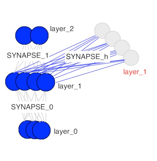
Big thing to take from this picture, there are only three weight matrices. Two of them should be very familiar (same names too). SYNAPSE_0 propagates the input data to the hidden layer. SYNAPSE_1 propagates the hidden layer to the output data. The new matrix (SYNAPSE_h....the recurrent one), propagates from the hidden layer (layer_1) to the hidden layer at the next timestep (still layer_1).

stop and make sure this feels comfortable in your mind

The gif above reflects the magic of recurrent networks, and several very, very important properties. It depicts 4 timesteps. The first is exclusively influenced by the input data. The second one is a mixture of the first and second inputs. This continues on. You should recognize that, in some way, network 4 is "full". Presumably, timestep 5 would have to choose which memories to keep and which ones to overwrite. This is very real. It's the notion of memory "capacity". As you might expect, bigger layers can hold more memories for a longer period of time. Also, this is when the network learns to forget irrelevant memories and remember important memories. What significant thing do you notice in timestep 3? Why is there more green in the hidden layer than the other colors?

Also notice that the hidden layer is the barrier between the input and the output. In reality, the output is no longer a pure function of the input. The input is just changing what's in the memory, and the output is exclusively based on the memory. Another interesting takeaway. If there was no input at timesteps 2,3,and 4, the hidden layer would still change from timestep to timestep.

i know i've been stopping... but really make sure you got that last bit


Part 3: Backpropagation Through Time:

So, how do recurrent neural networks learn? Check out this graphic. Black is the prediction, errors are bright yellow, derivatives are mustard colored.

They learn by fully propagating forward from 1 to 4 (through an entire sequence of arbitrary length), and then backpropagating all the derivatives from 4 back to 1. You can also pretend that it's just a funny shaped normal neural network, except that we're re-using the same weights (synapses 0,1,and h) in their respective places. Other than that, it's normal backpropagation.

Part 4: Our Toy Code

We're going to be using a recurrent neural network to model binary addition. Do you see the sequence below? What do the colored ones in squares at the top signify?

source: angelfire.com

The colorful 1s in boxes at the top signify the "carry bit". They "carry the one" when the sum overfows at each place. This is the tiny bit of memory that we're going to teach our neural network how to model. It's going to "carry the one" when the sum requires it. (click here to learn about when this happens)

So, binary addition moves from right to left, where we try to predict the number beneath the line given the numbers above the line. We want the neural network to move along the binary sequences and remember when it has carried the 1 and when it hasn't, so that it can make the correct prediction. Don't get too caught up in the problem. The network actually doesn't care too much. Just recognize that we're going to have two inputs at each time step, (either a one or a zero from each number begin added). These two inputs will be propagated to the hidden layer, which will have to remember whether or not we carry. The prediction will take all of this information into account to predict the correct bit at the given position (time step).

At this point, I recommend opening this page in two windows so that you can follow along with the line numbers in the code example at the top. That's how I wrote it.

Lines 0-2: Importing our dependencies and seeding the random number generator. We will only use numpy and copy. Numpy is for matrix algebra. Copy is to copy things.

Lines 4-11: Our nonlinearity and derivative. For details, please read this Neural Network Tutorial

Line 15: We're going to create a lookup table that maps from an integer to its binary representation. The binary representations will be our input and output data for each math problem we try to get the network to solve. This lookup table will be very helpful in converting from integers to bit strings.

Line 16: This is where I set the maximum length of the binary numbers we'll be adding. If I've done everything right, you can adjust this to add potentially very large numbers.

Line 18: This computes the largest number that is possible to represent with the binary length we chose

Line 19: This is a lookup table that maps from an integer to its binary representation. We copy it into the int2binary. This is kindof un-ncessary but I thought it made things more obvious looking.

Line 26: This is our learning rate.

Line 27: We are adding two numbers together, so we'll be feeding in two-bit strings one character at the time each. Thus, we need to have two inputs to the network (one for each of the numbers being added).

Line 28: This is the size of the hidden layer that will be storing our carry bit. Notice that it is way larger than it theoretically needs to be. Play with this and see how it affects the speed of convergence. Do larger hidden dimensions make things train faster or slower? More iterations or fewer?

Line 29: Well, we're only predicting the sum, which is one number. Thus, we only need one output

Line 33: This is the matrix of weights that connects our input layer and our hidden layer. Thus, it has "input_dim" rows and "hidden_dim" columns. (2 x 16 unless you change it). If you forgot what it does, look for it in the pictures in Part 2 of this blogpost.

Line 34: This is the matrix of weights that connects the hidden layer to the output layer. Thus, it has "hidden_dim" rows and "output_dim" columns. (16 x 1 unless you change it). If you forgot what it does, look for it in the pictures in Part 2 of this blogpost.

Line 35: This is the matrix of weights that connects the hidden layer in the previous time-step to the hidden layer in the current timestep. It also connects the hidden layer in the current timestep to the hidden layer in the next timestep (we keep using it). Thus, it has the dimensionality of "hidden_dim" rows and "hidden_dim" columns. (16 x 16 unless you change it). If you forgot what it does, look for it in the pictures in Part 2 of this blogpost.

Line 37 - 39: These store the weight updates that we would like to make for each of the weight matrices. After we've accumulated several weight updates, we'll actually update the matrices. More on this later.

Line 42: We're iterating over 100,000 training examples

Line 45: We're going to generate a random addition problem. So, we're initializing an integer randomly between 0 and half of the largest value we can represent. If we allowed the network to represent more than this, than adding two number could theoretically overflow (be a bigger number than we have bits to represent). Thus, we only add numbers that are less than half of the largest number we can represent.

Line 46: We lookup the binary form for "a_int" and store it in "a"

Line 48: Same thing as line 45, just getting another random number.

Line 49: Same thing as line 46, looking up the binary representation.

Line 52: We're computing what the correct answer should be for this addition

Line 53: Converting the true answer to its binary representation

Line 56: Initializing an empty binary array where we'll store the neural network's predictions (so we can see it at the end). You could get around doing this if you want...but i thought it made things more intuitive

Line 58: Resetting the error measure (which we use as a means to track convergence... see my tutorial on backpropagation and gradient descent to learn more about this)

Lines 60-61: These two lists will keep track of the layer 2 derivatives and layer 1 values at each time step.

Line 62: Time step zero has no previous hidden layer, so we initialize one that's off.

Line 65: This for loop iterates through the binary representation

Line 68: X is the same as "layer_0" in the pictures. X is a list of 2 numbers, one from a and one from b. It's indexed according to the "position" variable, but we index it in such a way that it goes from right to left. So, when position == 0, this is the farhest bit to the right in "a" and the farthest bit to the right in "b". When position equals 1, this shifts to the left one bit.

Line 69: Same indexing as line 62, but instead it's the value of the correct answer (either a 1 or a 0)

Line 72: This is the magic!!! Make sure you understand this line!!! To construct the hidden layer, we first do two things. First, we propagate from the input to the hidden layer (np.dot(X,synapse_0)). Then, we propagate from the previous hidden layer to the current hidden layer (np.dot(prev_layer_1, synapse_h)). Then WE SUM THESE TWO VECTORS!!!!... and pass through the sigmoid function.

So, how do we combine the information from the previous hidden layer and the input? After each has been propagated through its various matrices (read: interpretations), we sum the information.

Line 75: This should look very familiar. It's the same as previous tutorials. It propagates the hidden layer to the output to make a prediction

Line 78: Compute by how much the prediction missed

Line 79: We're going to store the derivative (mustard orange in the graphic above) in a list, holding the derivative at each timestep.

Line 80: Calculate the sum of the absolute errors so that we have a scalar error (to track propagation). We'll end up with a sum of the error at each binary position.

Line 83 Rounds the output (to a binary value, since it is between 0 and 1) and stores it in the designated slot of d.

Line 86 Copies the layer_1 value into an array so that at the next time step we can apply the hidden layer at the current one.

Line 90: So, we've done all the forward propagating for all the time steps, and we've computed the derivatives at the output layers and stored them in a list. Now we need to backpropagate, starting with the last timestep, backpropagating to the first

Line 92: Indexing the input data like we did before

Line 93: Selecting the current hidden layer from the list.

Line 94: Selecting the previous hidden layer from the list

Line 97: Selecting the current output error from the list

Line 99: this computes the current hidden layer error given the error at the hidden layer from the future and the error at the current output layer.

Line 102-104: Now that we have the derivatives backpropagated at this current time step, we can construct our weight updates (but not actually update the weights just yet). We don't actually update our weight matrices until after we've fully backpropagated everything. Why? Well, we use the weight matrices for the backpropagation. Thus, we don't want to go changing them yet until the actual backprop is done. See the backprop blog post for more details.

Line 109 - 115 Now that we've backpropped everything and created our weight updates. It's time to update our weights (and empty the update variables).

Line 118 - end Just some nice logging to show progress

Part 5: Questions / Comments

If you have questions or comments, tweet @iamtrask and I'll be happy to help.

Summary: Dropout is a vital feature in almost every state-of-the-art neural network implementation. This tutorial teaches how to install Dropout into a neural network in only a few lines of Python code. Those who walk through this tutorial will finish with a working Dropout implementation and will be empowered with the intuitions to install it and tune it in any neural network they encounter.

Followup Post: I intend to write a followup post to this one adding popular features leveraged by state-of-the-art approaches. I'll tweet it out when it's complete @iamtrask. Feel free to follow if you'd be interested in reading more and thanks for all the feedback!

Just Give Me The Code:

import numpy as np
X = np.array([ [0,0,1],[0,1,1],[1,0,1],[1,1,1] ])
y = np.array([[0,1,1,0]]).T
alpha,hidden_dim,dropout_percent,do_dropout = (0.5,4,0.2,True)
synapse_0 = 2*np.random.random((3,hidden_dim)) - 1
synapse_1 = 2*np.random.random((hidden_dim,1)) - 1
for j in xrange(60000):
layer_1 = (1/(1+np.exp(-(np.dot(X,synapse_0)))))
if(do_dropout):
layer_1 *= np.random.binomial([np.ones((len(X),hidden_dim))],1-dropout_percent)[0] * (1.0/(1-dropout_percent))
layer_2 = 1/(1+np.exp(-(np.dot(layer_1,synapse_1))))
layer_2_delta = (layer_2 - y)*(layer_2*(1-layer_2))
layer_1_delta = layer_2_delta.dot(synapse_1.T) * (layer_1 * (1-layer_1))
synapse_1 -= (alpha * layer_1.T.dot(layer_2_delta))
synapse_0 -= (alpha * X.T.dot(layer_1_delta))

Part 1: What is Dropout?

As discovered in the previous post, a neural network is a glorified search problem. Each node in the neural network is searching for correlation between the input data and the correct output data.

Consider the graphic above from the previous post. The line represents the error the network generates for every value of a particular weight. The low-points (READ: low error) in that line signify the weight "finding" points of correlation between the input and output data. The balls in the picture signify various weights. They are trying to find those low points.

Consider the color. The ball's initial positions are randomly generated (just like weights in a neural network). If two balls randomly start in the same colored zone, they will converge to the same point. This makes them redundant! They're wasting computation and memory! This is exactly what happens in neural networks.

Why Dropout: Dropout helps prevent weights from converging to identical positions. It does this by randomly turning nodes off when forward propagating. It then back-propagates with all the nodes turned on. Let���s take a closer look.

Part 2: How Do I Install and Tune Dropout?

The highlighted code above demonstrates how to install dropout. To perform dropout on a layer, you randomly set some of the layer's values to 0 during forward propagation. This is demonstrated on line 10.

Line 9: parameterizes using dropout at all. You see, you only want to use Dropout during training. Do not use it at runtime or on your testing dataset.

EDIT: Line 9: has a second portion to increase the size of the values being propagated forward. This happens in proportion to the number of values being turned off. A simple intuition is that if you're turning off half of your hidden layer, you want to double the values that ARE pushing forward so that the output compensates correctly. Many thanks to @karpathy for catching this one.

Tuning Best Practice

Line 4: parameterizes the dropout_percent. This affects the probability that any one node will be turned off. A good initial configuration for this for hidden layers is 50%. If applying dropout to an input layer, it's best to not exceed 25%.

Hinton advocates tuning dropout in conjunction with tuning the size of your hidden layer. Increase your hidden layer size(s) with dropout turned off until you perfectly fit your data. Then, using the same hidden layer size, train with dropout turned on. This should be a nearly optimal configuration. Turn off dropout as soon as you're done training and voila! You have a working neural network!

Want to Work in Machine Learning?

One of the best things you can do to learn Machine Learning is to have a job where you're practicing Machine Learning professionally. I'd encourage you to check out the positions at Digital Reasoning in your job hunt. If you have questions about any of the positions or about life at Digital Reasoning, feel free to send me a message on my LinkedIn. I'm happy to hear about where you want to go in life, and help you evaluate whether Digital Reasoning could be a good fit.

If none of the positions above feel like a good fit. Continue your search! Machine Learning expertise is one of the most valuable skills in the job market today, and there are many firms looking for practitioners. Perhaps some of these services below will help you in your hunt.

#indJobContent{padding-bottom: 5px;}#indJobContent .company_location{font-size: 11px;overflow: hidden;display:block;}#indJobContent.wide .job{display:block;float:left;margin-right: 5px;width: 135px;overflow: hidden}#indeed_widget_wrapper{position: relative;font-family: 'Helvetica Neue',Helvetica,Arial,sans-serif;font-size: 13px;font-weight: normal;line-height: 18px;padding: 10px;height: auto;overflow: hidden;}#indeed_widget_header{font-size:18px; padding-bottom: 5px; }#indeed_search_wrapper{clear: both;font-size: 12px;margin-top: 5px;padding-top: 5px;}#indeed_search_wrapper label{font-size: 12px;line-height: inherit;text-align: left; margin-right: 5px;}#indeed_search_wrapper input[type='text']{width: 100px; font-size: 11px; }#indeed_search_wrapper #qc{float:left;}#indeed_search_wrapper #lc{float:right;}#indeed_search_wrapper.stacked #qc, #indeed_search_wrapper.stacked #lc{float: none; clear: both;}#indeed_search_wrapper.stacked input[type='text']{width: 150px;}#indeed_search_wrapper.stacked label{display: block;padding-bottom: 5px;}#indeed_search_footer{width:295px; padding-top: 5px; clear: both;}#indeed_link{position: absolute;bottom: 1px;right: 5px;clear: both;font-size: 11px; }#indeed_link a{text-decoration: none;}#results .job{padding: 1px 0px;}#pagination { clear: both; }
#indeed_widget_wrapper{ width: 50%; height: 600px; background: #FFFFFF;}
#indeed_widget_wrapper{ border: 1px solid #DDDDDD; }
#indeed_widget_wrapper, #indeed_link a{ color: #000000;}
#indJobContent, #indeed_search_wrapper{ border-top: 1px solid #DDDDDD; }
#indJobContent a { color: #00c; }
#indeed_widget_header{ color: #000000; }





Machine Learning Jobs






What:
Where:








jobs by







View More Job Search Results