
Brian Potter's Blog
September 6, 2025
Reading List 09/06/2025
 EDF1 reactor in Chinon, France, via Works in Progress.
Welcome to the reading list, a weekly roundup of news and links related to buildings, infrastructure, and industrial technology. This week we look at London homebuilding, historical home prices, a humanoid robot loading a dishwasher, France’s history of nuclear reactor construction, and more. Roughly 2/3rds of the reading list is paywalled, so for full access become a paid subscriber.
Some housekeeping items this week:
The release date for the book has been pushed from September 23rd to October 14th, due to a shipping delay in Belgium.
The first chapter of the book is being previewed on Readwise.
No essay this week, but I’m finishing up a (very long) piece about the Manhattan Project that will be out next week.
Lars Doucet on property taxesRecently the idea that property taxes should be abolished seems to be gaining currency among conservatives. On substack, Lars Doucet of the Center for Land Economics has a good post on why this is both a bad idea and likely to fail:
In my home state of Texas, Republicans have tried and failed twice in back-to-back legislative sessions to eliminate property taxes. This is despite the fact that Texas has been under complete Republican domination for over twenty years.
First, it’s just too expensive. In 2024, the legislative budget board found that replacing property taxes would cost $81.5 billion dollars, more than the annual state budget of $72 billion. Read here:
“This is not something that you can find $81 billion on a per-year basis and not have a major impact on the remaining sales tax rates, because that is a huge amount of money to be able to replicate,” said state Sen. Paul Bettencourt, a Houston Republican and [Lt. Governor Dan] Patrick’s chief lieutenant on property taxes.
Second, replacing all property taxes with sales taxes would require raising the sales tax rate to over 19%, according to the Texas Taxpayers and Research Association. Just in case state leaders don’t think prices on everyday goods have risen high enough yet, they should note that inflation is the number one most important issue among Republicans.
It’s interesting that despite conservatives' frequent disdain for California, so many of them seem eager to replicate one of California’s biggest mistakes.
Also on the subject of property taxes, James Medlock on Twitter shares an interesting comparison of property taxes in absolute dollar terms (top) and as a percentage of home prices:
 Property taxes in dollars
 Property taxes as a % of home value.
It’s not clear to me why Texas and the great plains states have such high property taxes as a fraction of home value.
London homebuildingOn Twitter, Sam Hughes has a thread trying to diagnose the causes of London’s miserable record of recent homebuilding. In the first half of 2025, London had just 2158 housing starts (by contrast, Houston TX had around 24,000 building permits issued for single family homes alone in the same period). Part of this seems to be due to few applications getting approved:

I’ve previously noted that building regulations tend to be reflected in building layout in various ways: the distinct “layer cake” style of 1920s New York skyscrapers, for instance, is due to zoning regulations that required step-backs as a building got taller. Sam points to an aspect of this at work in London’s building shortage: a requirement that units be “dual aspect” (have windows on multiple facades):
 Historical home prices
The Philadelphia Federal Reserve bank has a really interesting data set that tracks the price of homes in 30 cities across the US going back to 1890. It’s based on analyzing 2.7 million listings from historical newspapers.

Expect to see an analysis of this data in a future newsletter.
Busiest flight routesWikipedia has an interesting list of the world’s busiest passenger flight routes. Lists of “biggest X” these days tend to be dominated by China, but air travel is a notable exception. China only has once airport in the top 10 busiest airports (Shanghai at #10), and only two of the busiest flight routes in the world are to Chinese cities.
The list isn’t what I expected: there are no US cities on the list at all, not even Los Angeles - San Francisco or New York - Washington. Possibly this is because traffic on these routes gets divided up between several different airports, or possibly the list is in error. The top routes are mostly southeast Asia: three in Japan, one in Korea, one in Vietnam. (Japan was initially surprising to me given its robust rail infrastructure, but the three routes are to cities on islands other than the main island.)


August 30, 2025
I Was Wrong About Data Center Water Consumption
(In lieu of a reading list this week, please enjoy this bonus essay about data center water consumption.)
In my essay on water usage in the US, I noted that “you need to be careful when talking about water use: it’s very easy to take figures out of context, or make misleading comparisons.”
I should have taken my own advice!
In the portion of the essay about data center water consumption, I state that the annual indirect water usage of data centers (from their share of power plant water usage) was around 579 million gallons a day, which I pulled from a Lawrence Berkeley Lab report on data centers. I assumed that this figure was total water use, and that because most power plant water use is non-consumptive, the actual water consumption was a small fraction of this (~19 million gallons). This, combined with the report’s estimate for water consumed by data centers directly, yielded a water consumption rate of around 66 million gallons a day.
But I didn’t read the report closely enough, and apparently this 579 million gallons a day was in fact consumptive use. This would increase the total consumptive water use of data centers from 66 million to 628 million, a huge difference.
However, an estimate of 579 million gallons a day of consumptive water use seems extremely high. Per the Berkeley Lab report, in 2023 all US data centers were estimated to consume 176 terawatt hours (TWh) of electricity, or around 4.4% of all electricity generated in the US. Per the USGS, the amount of water consumed (not merely used) by thermoelectric power plants in the US is around 1.2 million gallons a day per TWh for once-through cooling, and 1.4 million gallons a day per TWh for recirculating cooling.
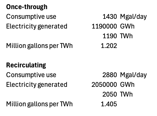
Even if we assume all data centers are powered by thermoelectric power plants, this implies a total indirect consumptive use for data centers of around 234 million gallons per day, substantially less than the 579 million gallons given by the LBL report. (The LBL report actually states “nearly 800 billion liters” in 2023, which works out to 579 million gallons daily use.)
It doesn’t seem to be a typo: later in the report they note that indirect water consumption from data center power use is around 4.5 liters per kilowatt/hour (which works out to 579 MGal/day), slightly higher than overall US electric power water consumption overall at 4.35 liters per kilowatt hour. 4.35 liters per kilowatt hour works out to 3.15 million gallons per day per TWh, more than twice the USGS value for thermoelectric power plant consumption (which as a reminder is 1.2-1.4 million gallons per day).
Why is the Berkeley Lab estimate for data center water consumption, and electric power water consumption more generally, so high?
A clue comes from a map the Berkeley Lab report includes on the water intensity of power generation. When we looked at water consumption of thermoelectric power plants, we noted that its concentrated in the eastern half of the country:
!function(){"use strict";window.addEventListener("message",(function(e){if(void 0!==e.data["datawrapper-height"]){var t=document.querySelectorAll("iframe");for(var a in e.data["datawrapper-height"])for(var r=0;r<t.length;r++){if(t[r].contentWindow===e.source)t[r].style.height=e.data["datawrapper-height"][a]+"px"}}}))}();However, per the Berkeley lab, the most intensive water use (in terms of liters per kilowatt hour) is found in the western half of the US (and to a lesser extent parts of the southeast). The areas of the country with really high amounts of thermoelectric power water consumption, by contrast — Texas, Florida, parts of the northeast — actually have some of the lowest water consumption on a kilowatt hour basis.
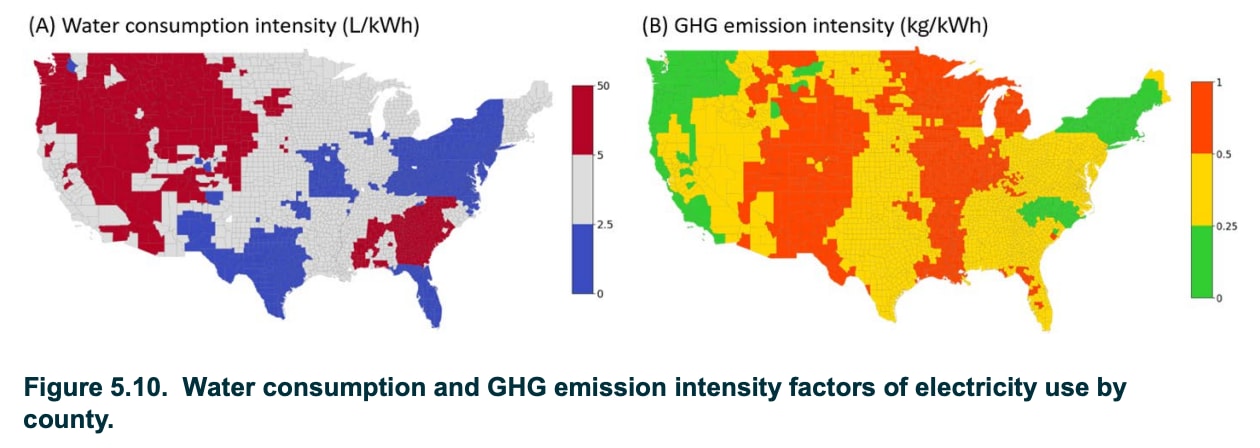
The answer appears to be that the Berkeley Lab report includes the effects of water evaporation from hydroelectric dam reservoirs in their water use calculations. The areas of the country with very intensive electric power water consumption (the northwest, the southwest, and the southeast) are areas with large amounts of hydropower (the Bonneville Power Administration, dams on the Colorado River, and the Tennessee Valley Authority).

Per this 2003 report from the National Renewable Energy Laboratory, thermoelectric power plants consume about 0.47 gallons of water per kilowatt hour of electricity generated, a figure that aligns with USGS values for thermal power plant water consumption. Hydroelectric power plants, on the other hand, “consume” an astounding 18.27 gallons per kilowatt hour via evaporation, almost 40 times as much! This value is so high that it drives up the average level of electric power water consumption for the entire US.

Does it make sense to include this water evaporation in the share of water consumed by data centers? I think it’s debatable. On the one hand, a huge dam reservoir does increase the level of water evaporation relative to an undammed river by increasing the amount of water surface area. On the other hand, some of this loss will be offset by the fact that dams make more fresh water available for use by storing excess in rainy seasons for use in drier seasons (this was part of the rationale for constructing several of the huge dams on the Colorado River, such as the Hoover and Grand Coulee Dams). And a dam that creates a reservoir as a supply of fresh water will have evaporation whether or not it generates electric power.
The NREL report notes these complexities:
There are substantial regional differences in the use of hydroelectric power, and therefore a thorough understanding of local conditions is necessary to properly interpret these data. There are river basins where evaporation is a substantial percentage of the total river flow, and this evaporation reduces the available supply both for downstream human consumption as well as having environmental consequences for coastal ecosystems that depend on fresh water supply. On the other hand, consider the case of a hydroelectric project on a relatively small river, which provides the fresh water supply to a major metropolitan area. In this case, the reservoir may be a valuable fresh water resource, especially if evaporation as a percentage of the river flow rate is low. If the downstream consequences for human consumption and coastal ecosystems are low, then the water consumption from hydroelectric projects would be irrelevant—whether or not electric generation occurs, the evaporation will still happen as a necessary consequence of providing fresh water supply to the region. These issues are beyond the scope of this paper, but must be considered when interpreting these results.
It’s not clear to me if the Berkeley Report tried to take this into account, but I suspect it didn’t, and merely applied estimates of regional hydroelectric evaporation without doing a dam-by-dam counterfactual of whether that evaporation would occur in the absence of electric power generation. (It’s worth noting here that the USGS doesn’t include hydroelectric evaporation when calculating US water use.)
Another issue I came across in the Berkeley Report is that it specifically excludes any sort of power purchase agreement, and instead estimates water consumption based on regional patterns of electricity generation.
It is important to note that the methodology used here to calculate indirect water and emission impacts does not incorporate any power purchase agreements between individual data center facilities and their electricity providers or on-site “behind the meter” generation, which could significantly affect water consumption and emissions estimates, depending on the electricity source. Nevertheless, due to the unavailability of facility-level data, we are constrained to assume the same electricity grid mix as that provided by the local balancing authority for all data centers within its jurisdiction.
This is a serious issue, because the hyperscalers (which currently are responsible for around 1/3 of all data center indirect water consumption) are very large purchasers of renewable energy via power purchase agreements. Amazon, Meta, Google, and Microsoft all report that 100% of their electricity comes from renewable sources. And outside of the hyperscalers, some large data center colocation companies are also very large purchasers of PPAs. Equinix, one of the largest data center leasing companies in the US, reported 96% renewable use in 2023. Digital Realty, another large data center operator, also uses PPAs to achieve 100% renewable use in North America. (This renewable use isn’t necessarily direct consumption: often it takes the form of companies buying certificates for power generated elsewhere, though many companies are also attempting to achieve direct renewable energy purchases).
The effect of PPAs on water consumption depends on the exact type of renewable energy used (and on how the renewable energy accounting is done). Solar and wind projects don’t use water during their operation, while nuclear power plants and (arguably) hydroelectric power plants do. In practice, most renewable PPAs by hyperscalars seem to be for wind or solar electricity.
ConclusionSo to wrap up, I misread the Berkeley Report and significantly underestimated US data center water consumption. If you simply take the Berkeley estimates directly, you get around 628 million gallons of water consumption per day for data centers, much higher than the 66-67 million gallons per day I originally stated.
However, the methods used to produce these estimates are debatable, and seem to have been chosen to give the maximum possible value for data center water consumption. If you exclude the water “consumed” by hydroelectric plants via reservoir evaporation, you get something closer to perhaps 275 million gallons per day.1 And if you take into account the fact that lots of data center operators use renewable energy PPAs (mostly from wind and solar sources), my guess is that you get something closer to 200-250 million gallons per day (though I haven’t run a detailed calculation here).
1275 million assumes that all power would come from thermoelectric plants, so the actual value would be somewhat less than this.
August 28, 2025
Ford and the Birth of the Model T
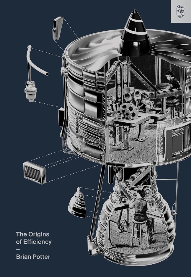
This is an excerpt from my forthcoming book, The Origins of Efficiency, out September 23rd.
Ford’s status as a large-volume car producer began with the predecessor to the Model T: the Model N, a four-cylinder, two-seater car initially priced at $500. At the time, the average car in the US cost more than $2,000, and it seemed nearly unimaginable that a car with the capabilities of the Model N could cost so little. In 1906, the year the Model N was introduced, Ford sold 8,500 of them, making the automaker bigger than the next two biggest car producers, Cadillac and Rambler, combined.
To produce such a huge volume of cars, Ford began to use many of the production methods it would develop more fully with the Model T. Many of the Model N’s parts were made of vanadium steel, a strong, lightweight, durable steel alloy. Vanadium steel allowed for a lighter car (the Model N weighed only 1,050 pounds), and was “machined readily.” This was important because Ford also made increasing use of advanced machine tools that allowed it to produce highly accurate interchangeable parts. In 1906, Ford advertised that it was “making 40,000 cylinders, 10,000 engines, 40,000 wheels, 20,000 axles, 10,000 bodies, 10,000 of every part that goes into the car…all exactly alike.” Only by producing interchangeable parts, Ford determined, could the company achieve high production volumes and low prices. Furthermore, Ford’s machine tools were arranged in order of assembly operations rather than by type, allowing parts to move from machine to machine with minimal handling and travel distance. It also made extensive use of production aids such as jigs, fixtures, and templates. These “farmer tools”—so called because they supposedly made it possible for unskilled farmers to do machining work—greatly simplified Ford’s machining operations.
The Model N was so popular that demand exceeded capacity, which allowed Ford to plan production far in advance. This meant Ford could purchase parts and materials in large quantities at better prices and schedule regular deliveries, ensuring a steady, reliable delivery of material, which allowed it to maintain just a 10-day supply of parts on hand.
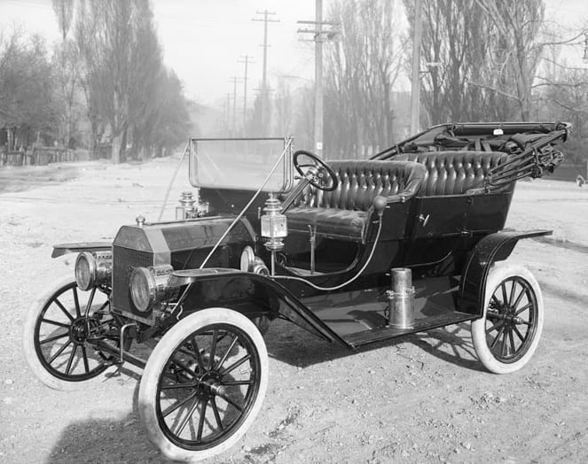
But even as the Model N became Ford’s bestseller, the company was designing the car that would supersede it: the Model T. In addition to improving upon many aspects of the Model N— the Model T would be a five-seater, include a new transmission that made it easier to shift gears, and have a three-point suspension that made it better able to navigate America’s low-quality roads—the Model T’s design also involved significant process improvements. For one, it pushed the machining precision of the Model N even further. In his history of Ford, Douglas Brinkley notes that “in an industry previously unfettered by anything like exacting measurements, the typical tolerance on the Model T was 1/64th of an inch.” Indeed, outside the auto industry, some types of manufacturing were done without even the aid of dimensioned drawings. This precision machining was “the rock upon which mass production of the Model T was based.” Not only did a high level of precision facilitate manufacturing, it also made for a better product—one that was much more reliable than any other car on the market. Because parts were interchangeable, repairs were simpler. And the precision of the machining meant that unlike most other automakers, Ford didn’t need to test the engine before it was attached to the chassis, since “if parts were made correctly and put together correctly, the end product would be correct.” The Model T would ultimately cost around $100 a year to maintain, at a time when the maintenance of other cars cost $1,500 per year.
At the time, most four-cylinder engines were cast either as four separate cylinders or two groups of two cylinders and then attached together, which required extra time and material. The Model T’s engine block, on the other hand, was cast as a single piece. Several components—the rear axle housing, transmission housing, and crankcase—were not made of the more customary cast steel but rather stamped steel, a then-novel technology for automobiles that was cheaper than casting. Like any new technology, these production methods required time and effort to implement—it took 11 months of development to figure out how to produce the drawn steel crankcase—but the manufacturing cost savings were worth the effort. Over time, more and more Model T parts would be made from pressed steel, though the transmission housing itself was later changed to cast aluminum.
The Model T was not the cheapest car on the road when it was introduced—at $850, it cost several hundred dollars more than the Model N. But even when Ford later briefly raised the price to over $900, no other car offered so many features for the same price. Between October 1908, when the new model was announced, and September of the following year, Ford sold 10,607 Model Ts. By March, Ford had temporarily stopped allowing orders because it had filled its factory capacity until August.
As production for the Model T began, Ford was already busy reworking and improving the production system. Originally, cars were transported by rail to Ford dealerships all over the country. But, realizing this wasted train space, Ford soon began to create local assembly plants. Model T parts would be shipped to these plants and then assembled into cars, dramatically lowering shipping costs. In his history of the company, Allan Nevins notes that “by shipping parts in a knocked-down state, [Ford] was able to load the components of twenty-six Model Ts into an ordinary freight car instead of the three or four complete cars that could otherwise be sent.” And while the Model T had originally come in several different colors, in 1912 Ford announced that the Model T would now come in a single color: black.
The first Model Ts were assembled in Ford’s Piquette Avenue plant in Detroit, which was built in 1904. But in 1910 it moved production to the new, larger Highland Park factory, also in Michigan, which was considered to be the best designed factory in the world. At a time when electricity was still somewhat uncommon in manufacturing, electric motors drove mechanical belting and overhead cranes were used to move material. At the Piquette Avenue plant, material came in on the bottom floor and final assembly was done on the top floor. But at Highland Park, material came in on the top floor and gradually moved down to assembly on the ground floor. To facilitate the movement of material, thousands of holes were cut in the floor, which allowed parts to move down through the factory through chutes, conveyors, and tubes.
At Piquette Avenue, machine tool use had been extensive, but the machinery was largely general-purpose. With the decision to focus on a single model and the subsequent enormous increase in production volume, Ford began to buy or create dozens of special-purpose machine tools designed specifically for the Model T, such as a machine for automatically painting wheels and another for drilling holes in a cylinder block. As with the farmer tools first introduced on the Model N, these special-purpose tools not only produced parts more cheaply but could also be operated by less-skilled machinists, reducing labor costs.
It was only the enormous production volumes of the Model T that enabled Ford to make such extensive use of special-purpose machinery. Similarly, it was only by virtue of its large volumes that Ford could afford to purchase dedicated steel-stamping presses to churn out pressed-steel crankcases, which were cheaper and used less material than the cast iron employed by other manufacturers.
Ford experimented with machinery continuously, and the factory was in a constant state of rearrangement as new machinery was brought online and old machinery was scrapped. In some cases, machines that were just a month old were replaced with newer, better ones. By 1914, Highland Park had 15,000 machine tools. As at other automakers, machinery was packed close together in the order that operations were performed. But Ford took this concept much further, sandwiching drilling machines and even carbonizing furnaces between heavy millers and press punches. Not only did this machine placement for material flow keep handling to a minimum, but the tight packing of machinery also prevented inventory from building up in the factory.
Ford’s process improvements weren’t limited to new and better machine tools. The company constantly examined its operations to figure out how they could be done in fewer steps. In one case, a part being machined on a lathe required four thumbscrews to attach it to the lathe, each of which had to be twisted into place to position the part and untwisted to remove it. By designing a special spindle with an automatic clamp for the part, Ford reduced the time to perform the operation by 90 percent.
The Model T itself was continuously redesigned to reduce costs. When the stamped-steel axle housing proved complex to manufacture, it was redesigned to be simpler. Brass carburetors and lamps were replaced by cheaper ones made of iron and steel. A water pump that was found to be extraneous was removed. As a result of these constant improvements, Ford was able to continuously drop the price. By 1911, the cost of a Touring model had fallen to $780; by 1913, it had dipped to $600. And as costs fell, sales rose. In 1911, Ford sold 78,000 Model Ts. In 1912, it sold 168,000. And in 1913, it sold 248,000.
Then, in 1913, Ford began to install the system that would become synonymous with mass production: the assembly line. Though gravity slides and conveyors had existed prior to 1913, Ford hadn’t yet developed a systematic method for continuously moving the work to the worker during assembly. The first assembly line was installed in the flywheel magneto department. Previously, workers had stood at individual workbenches, each assembling an entire flywheel magneto. But on April 1, 1913, Ford replaced the workbenches with a single steel frame with sliding surfaces on top. Workers were instructed to stand in a designated spot and, rather than assemble an entire magneto, perform one small action, then slide the work down to the next worker, repeating the process over and over.
The results spoke for themselves. Prior to the assembly line, it took a single worker an average of 20 minutes to assemble a flywheel magneto. With the assembly line, it took just over 13 minutes.
Ford quickly found even more ways to improve the process. To prevent workers from having to bend over, the height of the line was raised several inches. Moving the work in a continuous chain allowed it to be synchronized, which sped up the slow workers and slowed down the fast ones to an optimal pace. Within a year, the assembly time for flywheel magnetos had fallen to five minutes.
This experiment in magneto assembly was quickly replicated in other departments. In June 1913, Ford installed a transmission assembly line, bringing assembly time down from 18 minutes to nine. In November, the company installed a line for the entire engine, slashing assembly time from 594 minutes to 226 minutes. As with the flywheel magneto, further adjustments and refinements to the lines yielded even greater productivity gains. In August, Ford began to create an assembly line for the entire chassis. Its first attempt, using a rope and hand crank to pull along the car frames, dropped assembly time from 12.5 hours to just under six. By October, the line had been lengthened and assembly time had fallen to three hours. By April 1914, after months of experimentation, car assembly time had been cut down to 93 minutes.
In addition to reducing assembly times, the assembly line decreased inventories. By moving the work continuously along the line, there was no opportunity for parts to accumulate in piles near workstations. The Highland Park facility kept enough parts on hand to produce 3,000 to 5,000 cars—just six to 10 days’ worth of production. This was only possible through careful control of material deliveries and precise timing of the different assembly lines.
As the assembly lines were installed, Ford continued to make other process improvements. Operations were constantly redesigned to require fewer production steps. One new machine reduced the number of operations required to install the steering arm to the stub axle from three to one. An analysis of a piston rod assembly found that workers spent almost 50 percent of their time walking back and forth. When the operation was redesigned to reduce time spent moving about, productivity increased 50 percent. A redesigned foundry that used molds mounted to a continuously moving conveyor belt not only increased assembly speed but also allowed the use of less-skilled labor in its operation.
Meanwhile, Ford continued to tweak the design of the Model T. The body was redesigned to be simpler and less expensive to produce. Costly forged parts were eliminated by combining them with other components. Fastener counts were reduced. By 1913, comparable cars to the Model T cost nearly twice as much as the Model T did. And the price continued to fall. By 1916, the cost had dropped to just $360—a two-thirds reduction in just six years.
With the Model T, Ford didn’t just create a cheap, practical car. It built an efficiency engine. With high-precision machining, Ford was able to manufacture highly accurate parts that resulted in a better, more reliable car, required less work to assemble, and used less-skilled labor. This made the car inexpensive, which, along with its excellent design, resulted in sky-high demand. High demand and high production volume enabled Ford to make additional process improvements. It designed and deployed special-purpose machine tools—large fixed costs that were only practical at huge production volumes—which increased production rates and decreased labor costs. It set up dedicated assembly plants (also large fixed costs), which enabled substantial reductions in transportation costs. It built a new factory (another large fixed cost) specially designed to optimize the flow of production. It placed massive material orders, resulting in lower prices, lower inventory costs, and smoother material delivery, reducing variability and making maximum use of production facilities. And, as all these improvements drove down the cost of the car, demand for the Model T continued to rise, enabling Ford to improve its processes even more.
More generally, the high production volumes of the Model T made any process improvement incredibly lucrative. Even a small change had a big impact when multiplied over hundreds of thousands of Model Ts. Consider, for instance, the effect of one minor improvement among many, the removal of a forged bracket:
Presume that it took just one minute to install the forged brackets on each chassis. Ford produced about 200,000 cars in 1914. It would have taken 200,000 minutes, or better than 3,300 hours for the installation of these forgings. Each of these brackets was held in place with three screws, three nuts, and three cotter pins; that’s six screws and nuts per car—1,200,000 of each! This saving does not take into account the cotter keys nor the brackets themselves. Each bracket had four holes which had to be drilled— 1,600,000 holes—which took some time as well. If the screws alone were as cheap as ten for a penny, the savings on screws alone would have been $1,200!
Since any production step would be repeated millions of times, it was worth carefully studying even the smallest step for possible improvements. This resulted in an environment of continuous improvement, where processes were constantly experimented on, tweaked, ripped out, and replaced with better ones. Ford could, and often did, experiment with and create designs for its own machine tools, only later having a tool builder supply them. And if new machines didn’t work properly, Ford could afford to abandon the experiment. In 1916, a custom-designed piston-making machine that cost $180,000 to produce—$5 million in 2023 dollars—was “thrown into the yard” after repeated failures and replaced with simple lathes.
The ultimate example of this environment of constant tinkering is the assembly line, which took years of experimentation to fully work out and required restructuring almost all of Ford’s operations. By breaking down operations into a series of carefully sequenced steps and mechanically moving material through them, Ford was able to eliminate extraneous operations, reduce inventories, and increase production rates, enabling even lower costs and greater scale. This entire chain of improvements was itself made possible by the development of precision-machined parts.
The Model T would change the world, both by making the car a ubiquitous feature of American life and, more subtly but no less significantly, showing what could be achieved with large-volume production and a cascading chain of improvements.
The Origins of Efficiency is available for preorder at Amazon, Stripe Press, Barnes and Noble, and Bookshop. It will be out September 23rd.
August 23, 2025
Reading List 08/23/25
 Palais de Justice, Bordeaux, France, via @sci_fi_infra.
Welcome to the reading list, a weekly roundup of news and links related to buildings, infrastructure, and industrial technology. This week we look at thermal energy storage, an adjustable allen wrench, the new race to the moon, the former world’s largest indoor water park, and more. Roughly 2/3rds of the reading list is paywalled, so for full access become a paid subscriber.
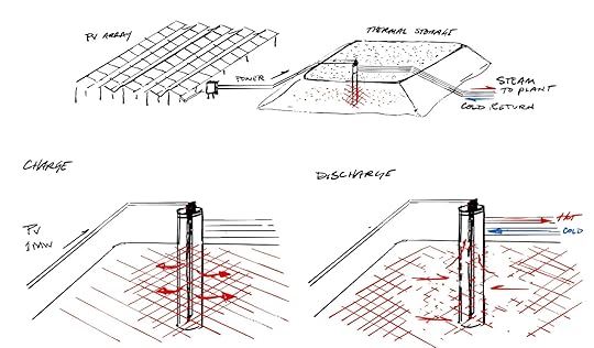
Standard ThermalFriend of the newsletter Austin Vernon’s company, Standard Thermal, just emerged from stealth. It aims to achieve extremely low long-term energy storage costs by using electricity from solar PV to heat up huge mounds of dirt. From Austin’s substack:
The purpose of Standard Thermal is to make energy from solar PV available 24/7/365 at a price that is competitive with US natural gas.
Our technology works by storing energy as heat in the least expensive storage material available - large piles of dirt. Co-located solar PV arrays provide energy (as electricity) and are simpler and cheaper than grid-connected solar farms. Electric heating elements embedded in the dirt piles convert electricity to heat. Pipes run through the pile, and fluid flowing through them removes heat to supply the customer. The capital cost, not including the solar PV, is comparable to natural gas storage at less than $0.10/kilowatt-hour thermal and 1000x cheaper than batteries.
These are the customer archetypes we can save the most money for right now:
Solar developers with oversized arrays greater than 300 kilowatts and heat demand at the location. Our system can store the summer excess production for winter thermal demand.
Isolated energy users forced to use propane or fuel oil, typically using more than 50,000 gallons of propane per year.
England drought
The storage system can provide hundreds of megawatts of thermal demand as long as land is available…

England is apparently in the midst of a major drought. Rainfall levels are below average, and reservoir levels have fallen. Many water providers have implemented a ban on using hoses for watering lawns or gardens, and restrictions might get more severe. Via the Guardian:
The National Drought Group met to discuss actions to save water across the country, and Steve Reed, the environment secretary, briefed the chancellor of the duchy of Lancaster, Pat McFadden, about the risks posed by the dry weather.
Water companies are preparing to take more drastic measures to conserve water as supplies dwindle.
Southern Water, some of whose customers are already under a hosepipe ban, has applied for a non-essential use ban that would prohibit businesses from taking actions such as filling swimming pools or cleaning their windows.
The company has also applied for an emergency order to take water from a rare chalk stream after it drops below its ecologically safe water flow.
The drought is hitting many sectors across the country, with many canals shut to navigation due to low water levels, farmers struggling to grow crops and feed livestock, and higher numbers of fish die-offs being reported by anglers and others who use England’s rivers.
Two rivers, the Wye and the Great Ouse at Ely, were at their lowest on record for July, and only 89% of long-term average rainfall was recorded for the month across England. This is the sixth consecutive month of below-average rainfall.
This BBC article has some good graphics illustrating various aspects of the drought:

Reservoir levels are also low:
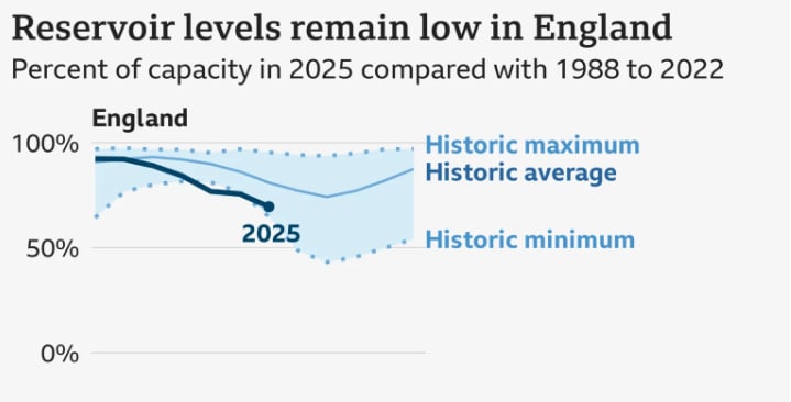
(I had originally described England as “famously rainy”, but apparently its only ranked number 78 in annual average precipitation. Colombia is #1.)
Related, apparently it’s been 30 years since a new water storage reservoir was built in England.
In an extremely misguided attempt to deal with the water shortage, the UK Government recommended that people delete files off the cloud to reduce load on data centers.
AI environmental impactOn the subject of data center water consumption, earlier this week Google released a paper that analyzes the environmental cost of its “Gemini” AI model. Per Google, the median Gemini response uses 0.24 watt-hours of electricity (equivalent to running a 60-watt lightbulb for about 15 seconds) and 0.26 milliliters of water (about 5 drops).
AI is unlocking scientific breakthroughs, improving healthcare and education, and could add trillions to the global economy. Understanding AI’s footprint is crucial, yet thorough data on the energy and environmental impact of AI inference — the use of a trained AI model to make predictions or generate text or images — has been limited. As more users use AI systems, the importance of inference efficiency rises.
That’s why we’re releasing a technical paper detailing our comprehensive methodology for measuring the energy, emissions, and water impact of Gemini prompts. Using this methodology, we estimate the median Gemini Apps text prompt uses 0.24 watt-hours (Wh) of energy, emits 0.03 grams of carbon dioxide equivalent (gCO2e), and consumes 0.26 milliliters (or about five drops) of water1 — figures that are substantially lower than many public estimates. The per-prompt energy impact is equivalent to watching TV for less than nine seconds.
At the same time, our AI systems are becoming more efficient through research innovations and software and hardware efficiency improvements. For example, over a recent 12 month period, the energy and total carbon footprint of the median Gemini Apps text prompt dropped by 33x and 44x, respectively, all while delivering higher quality responses.
Some folks have criticized this work for only including direct water use, and not including indirect water use required to generate the electricity used. But as we noted in this week’s essay about US water use, the vast majority of water used for electricity generation is non-consumptive, so this wouldn’t have much of an impact on consumptive water use.
Adjustable allen wrenchChronova Engineering (a YouTube channel we’ve featured before for building the world’s smallest electric motor) has a video showing the construction of an adjustable allen wrench. Adjustable wrenches are of course incredibly common, but this appears to be the first time someone has built an adjustable allen wrench (though it wouldn’t surprise me if prior art exists somewhere).
It turns out that the nature of an allen wrench — which grips a fastener from the inside, and places a large amount of torque along a slender shaft — makes building an adjustable one difficult. The wrench only ends up being adjustable over a relatively short range, 4 mm to 6 mm, and has a fairly bulbous head that prevents access in tight places.

If you’re interested in building one, the 3D files and CAD drawings are available on their (paywalled) Patreon page.
August 21, 2025
How Does the US Use Water?
Water infrastructure often gets less attention and focus than other types of infrastructure. Both the Federal Highway Administration and the Department of Energy have annual budgets around $46 billion dollars. The Department of Housing and Urban Development has an annual budget of $60 billion. The closest thing the federal government has to a department of water infrastructure, the Bureau of Reclamation, has an annual budget of just $1.1 billion. Water in the US is generally both widely available and inexpensive: my monthly water bill is roughly 5% of the cost of my monthly electricity bill, and the service is far more reliable. And unlike, say, energy, water isn’t the locus of exciting technological change or great power competition.
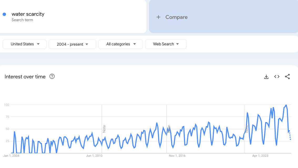
But this might be changing. Rising demand for water in the arid southwest (which has experienced decades of drought) is creating increasing concern about water availability. Vast amounts of investment is being poured into data center construction, and while data centers are most notable for consuming large amounts of power, they’re also heavy users of water: a large data center can use millions of gallons of water a day for cooling. Google search interest for “water scarcity” has gradually risen over the last two decades.
 Via Google Trends.
Because water is such a critical resource, needed for everything from agriculture to manufacturing to artificial intelligence to sustaining basic human life, it's worth understanding how we use water, and how that use has changed over time.
Overview of US water useMost of us probably remember learning about the water cycle in school. Water falls to the earth via precipitation — rain, snow, sleet — and flows into rivers, lakes, streams, and water-bearing geological strata called aquifers. From there, water continues to move: it goes back into the atmosphere via evapotranspiration, moves from streams and rivers into aquifers (and vice versa), and flows out into the ocean.1
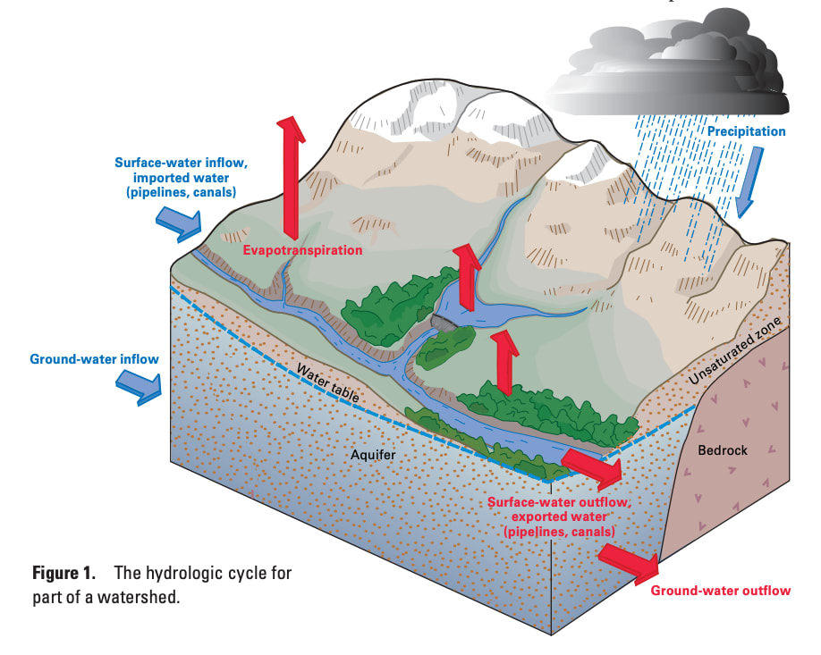 Water cycle, via USGS.
Altogether, the US receives about 5 trillion gallons of precipitation a day. Most of that (63%) gets returned to the atmosphere via evapotranspiration. Much of the rest ultimately flows into the Gulf of Mexico (11%), Pacific Ocean (6%), and Atlantic Ocean (2%). About 10% gets stored in surface bodies of water (lakes, reservoirs) or underground aquifers, and 6% flows back into Canada. The remaining 2% is consumed by people in various ways.
 Via USGS.
We use water by tapping these various stores and flows. At a high level, water infrastructure resembles electricity infrastructure. In both cases, you have large sources of supply (power plants for electricity and lakes/rivers/underground aquifers for water), which gets transported by a high-capacity transmission system. With electricity transmission is done by high-voltage power lines which connect power plants to substations; with water it's done by large-diameter pipes which connect sources to treatment plants or water storage facilities. From there, as with electricity, water is moved by a distribution system, smaller-capacity pipes and pumps that bring water to individual homes and businesses. And as with electricity, very large consumers of water (along with some smaller consumers) might tap various sources of water directly rather than get their supply via a utility company.
 Water infrastructure and use, via USGS.
 Schematic of a water supply system, from Water Distribution System Operation and Maintenance.Water use by category
As of 2015, the year of the most recent USGS report on US water consumption, the US used about 322 billion gallons of water each day, or 117 trillion gallons each year. 87% of this is freshwater, and the rest is saltwater, either from the ocean or from brackish coastal water like estuaries. 74% of all US water use is from surface sources like lakes and rivers, and 26% is from underground aquifers.
!function(){"use strict";window.addEventListener("message",(function(e){if(void 0!==e.data["datawrapper-height"]){var t=document.querySelectorAll("iframe");for(var a in e.data["datawrapper-height"])for(var r=0;r<t.length;r++){if(t[r].contentWindow===e.source)t[r].style.height=e.data["datawrapper-height"][a]+"px"}}}))}();An important distinction when understanding water use is “consumptive” vs “non-consumptive” uses. Consumptive water use is when the water is consumed as part of the process: either it gets incorporated into whatever is being produced, evaporates back into the atmosphere, or is otherwise no longer available in fluid form. Non-consumptive water use is when the water is still available to use in fluid form after the process is completed, though perhaps at a higher temperature, or with some additional pollutants or impurities. The graph below shows total water use by category, broken out into consumptive and non-consumptive uses:
!function(){"use strict";window.addEventListener("message",(function(e){if(void 0!==e.data["datawrapper-height"]){var t=document.querySelectorAll("iframe");for(var a in e.data["datawrapper-height"])for(var r=0;r<t.length;r++){if(t[r].contentWindow===e.source)t[r].style.height=e.data["datawrapper-height"][a]+"px"}}}))}();As of 2015, the largest user of water in the US is actually thermoelectric power plants — plants that use heat to produce steam to drive a turbine. Water is used in these plants to condense steam back to liquid water so that it can be heated again and routed back through the turbine. Thermoelectric power plants make up 41% of total water use in the US. However, nearly all this (around 97%) use is non-consumptive. Historically thermoelectric power plants were built using “once-through” cooling systems: water would be drawn from some source, run through the cooling system, and then dumped back out into the same source at a slightly raised temperature. This water can be either fresh water or saltwater, and around 97% of the saltwater used in the US each year is used to cool coastal power plants.
 Via EIA.
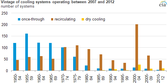
Since the 1970s, most thermoelectric power plants have been built with recirculating cooling systems rather than once-through cooling systems. This is due to things like the Clean Water Act, which set limits on thermal discharge from power plants and made once-through cooling systems less attractive. Recirculating systems circulate the same water over and over again through the system. These systems use much less water overall, but a much greater fraction of the water they do use is consumed (it's lost to evaporation, typically via large cooling towers). As of 2012 about 43% of thermal power plants used once-through cooling, but once-through cooling systems make up around 96% of all water used by thermoelectric power plants.
!function(){"use strict";window.addEventListener("message",(function(e){if(void 0!==e.data["datawrapper-height"]){var t=document.querySelectorAll("iframe");for(var a in e.data["datawrapper-height"])for(var r=0;r<t.length;r++){if(t[r].contentWindow===e.source)t[r].style.height=e.data["datawrapper-height"][a]+"px"}}}))}();After power plants, the next largest use of water in the US is for irrigation: watering plants and crops. Altogether, irrigation makes up 37% of total US water use. Unlike thermoelectric power plants, most of this water (just over 60%) is consumptive use. What’s more, even the irrigation water that isn’t consumed may not be readily reused. While thermoelectric plants which typically dump their water back into the same river, lake, or ocean it was drawn from, much of the non-consumptive water used for irrigation seeps back into the ground, potentially far from where it was originally tapped. Depending on how water flows through the ground in a particular location, it could be centuries or even longer before that water reaches somewhere it can be easily retrieved.
Most water for irrigation is used for crops, though it’s hard to know exactly what fraction, as many states don’t break out irrigated cropland as a separate category.2 As of 2015, the US has around 63 million acres of irrigated land. This is around 20% of the US’s 337 million acres of cropland, but it’s responsible for around 54% of the value of US crops. The largest water-using crop in the US is alfalfa (around 11.1 billion gallons per day), followed by orchards (10.9 billion), corn (10.4 billion), soybeans (5.1 billion), and rice (5 billion) (though if we lump all separate categories of corn together — sweet corn, silage, etc. —, it comes in at number one).
!function(){"use strict";window.addEventListener("message",(function(e){if(void 0!==e.data["datawrapper-height"]){var t=document.querySelectorAll("iframe");for(var a in e.data["datawrapper-height"])for(var r=0;r<t.length;r++){if(t[r].contentWindow===e.source)t[r].style.height=e.data["datawrapper-height"][a]+"px"}}}))}();Another user of irrigation water is golf courses. The US has around 16,000 golf courses, and collectively they use about a billion gallons of water a day, or around 0.3% of total US water use.
After irrigation, the next largest category of US water use is public utility supplied water for homes and businesses. Public water use totals to around 39 billion gallons a day, or 12% of total US water use. Most public water — 23.3 billion gallons, or around 60% — is for domestic use in homes. In addition to publicly supplied water for homes, another 3.3 billion gallons are self-supplied to homes via things like privately owned wells. An estimated 42 million people in the US use self-supplied water.
Average per-capita domestic water use in the US is 82 gallons per day. By comparison, German homes use around 33 gallons per person per day, UK homes use around 37 gallons, and French homes use around 39 gallons.
The next largest category of water use is industry, which uses about 14.8 billion gallons of water a day, or 4.5% of all US water use). Many industrial processes require large amounts of water, often either for cooling or as a way to carry and mix materials or chemicals. The chart below shows several US industries that use large amounts of water.
!function(){"use strict";window.addEventListener("message",(function(e){if(void 0!==e.data["datawrapper-height"]){var t=document.querySelectorAll("iframe");for(var a in e.data["datawrapper-height"])for(var r=0;r<t.length;r++){if(t[r].contentWindow===e.source)t[r].style.height=e.data["datawrapper-height"][a]+"px"}}}))}();One of the largest water-using industries is forest products, particularly pulp and paper mills which require water for things like rinsing the pulp after it's been bleached. Forest product manufacturing in the US uses around 4 billion gallons of water a day. Other large industrial users of water are steelmaking (around 1.8 billion gallons per day), crude oil refining (around 270 million gallons a day), and semiconductor manufacturing (around 80 million gallons a day).
However, as with thermoelectric power plants, much of industrial water use is non-consumptive (though USGS doesn’t break out consumptive and non-consumptive separately for industrial use). In forest products, most of the water is returned to the source after it goes through the process, and only around 12% of the water used is consumptive. Similarly, only around 10% of the water used for steel production is consumed.
Because of rising concern about water use of data centers, it's worth looking at them specifically. Per Lawrence Berkeley Lab, in 2023, data centers used around 48 million gallons of water a day directly for cooling. Most of this water will evaporate as part of the cooling process, and is thus consumed. If you include indirect water use by including their share of water required for electricity consumption, this adds another 580 million gallons per day. However, as we’ve noted, most thermoelectric power plant water use is not consumptive. Taking this into account, actual water consumed by data centers is around 66 million gallons per day. By 2028, that’s estimated to rise by two to four times.
!function(){"use strict";window.addEventListener("message",(function(e){if(void 0!==e.data["datawrapper-height"]){var t=document.querySelectorAll("iframe");for(var a in e.data["datawrapper-height"])for(var r=0;r<t.length;r++){if(t[r].contentWindow===e.source)t[r].style.height=e.data["datawrapper-height"][a]+"px"}}}))}();This is a large amount of water when compared to the amount of water homes use, but it's not particularly large when compared to other large-scale industrial uses. 66 million gallons per day is about 6% of the water used by US golf courses, and it's about 3% of the water used to grow cotton in 2023.
We can also think about it in economic terms. The 2.5 billion gallons per day required to grow cotton in the US created about six billion pounds of cotton in 2023, worth around $4.5 billion. Data centers, by contrast, are critical infrastructure for technology companies worth many trillions of dollars. Anthropic alone, just one of many AI companies, is already making $5 billion dollars every year selling access to its AI model. A gallon of water used to cool a data center is creating thousands of times more value than if that gallon were used to water a cotton plant.
The remaining users of water in the US are aquaculture (fish farms) at 7.5 billion gallons a day (2.3% of all water use), mining at 4 billion gallons a day (1.2%), and water for livestock at 2 billion gallons a day (0.6%).
Water use by geographyHow does US water use vary by geography? The map below shows total water consumption by state:
!function(){"use strict";window.addEventListener("message",(function(e){if(void 0!==e.data["datawrapper-height"]){var t=document.querySelectorAll("iframe");for(var a in e.data["datawrapper-height"])for(var r=0;r<t.length;r++){if(t[r].contentWindow===e.source)t[r].style.height=e.data["datawrapper-height"][a]+"px"}}}))}();California is the number one water consumer at 28.8 billion gallons per day, followed by Texas (21.3 billion), Idaho (17.7 billion), Florida (15.3 billion) and Arkansas (13.8). The large consumers of water are states that either have a lot of irrigated land (California, Idaho, Arkansas), have a lot of thermal power plant cooling (Florida), or both (Texas).
 Via USGS.
Because this lumps in such disparate uses of water, it's more illuminating to break this down by category. The map below shows water used for irrigation by state.
!function(){"use strict";window.addEventListener("message",(function(e){if(void 0!==e.data["datawrapper-height"]){var t=document.querySelectorAll("iframe");for(var a in e.data["datawrapper-height"])for(var r=0;r<t.length;r++){if(t[r].contentWindow===e.source)t[r].style.height=e.data["datawrapper-height"][a]+"px"}}}))}();And this map shows a more granular view of where, specifically, irrigated acres are located.
 Via USDA.
Most irrigated acres are in the western half of the US. This isn’t that surprising, as western states get far less precipitation than eastern states. The map below shows average yearly precipitation by state (averaged between the years 1971 and 2000).
!function(){"use strict";window.addEventListener("message",(function(e){if(void 0!==e.data["datawrapper-height"]){var t=document.querySelectorAll("iframe");for(var a in e.data["datawrapper-height"])for(var r=0;r<t.length;r++){if(t[r].contentWindow===e.source)t[r].style.height=e.data["datawrapper-height"][a]+"px"}}}))}();Average annual rainfall is around 45.6 inches per year in the eastern half of the US, compared to 21 inches per year in the western half.
The amount of water an individual state has available for productive use is not simply a portion of all the precipitation it receives (due to movement of water through rivers, streams and aquifers), but it's nevertheless interesting to see irrigation water use as a fraction of a state’s total precipitation.
!function(){"use strict";window.addEventListener("message",(function(e){if(void 0!==e.data["datawrapper-height"]){var t=document.querySelectorAll("iframe");for(var a in e.data["datawrapper-height"])for(var r=0;r<t.length;r++){if(t[r].contentWindow===e.source)t[r].style.height=e.data["datawrapper-height"][a]+"px"}}}))}();In most states, irrigation water is equivalent to a tiny fraction of total precipitation: in 30 states it's less than 1%. But in some western states it's much higher. In Idaho water used for irrigation is equivalent to more than 20% of all the precipitation the state receives.
Outside of the western states, the major user of irrigation water is Arkansas. Apparently this is due to the large amount of rice cultivated there (nearly half of all rice produced in the US), which requires a very large amount of water to produce.
Much of the water used for irrigation — roughly half — is pumped from underground aquifers. In many places in the US, groundwater is being pumped out faster than it recharges from precipitation, leading to gradual depletion of the aquifer.
 Groundwater depletion in US aquifers, via USGS.
(Interestingly, this map shows groundwater recharging in an Idaho aquifer, despite Idaho being such a large user of irrigation water. Possibly this is explained by the time period difference, as this map only goes to 2008.)
Other than irrigation, the largest category of water use in the US is cooling at thermoelectric power plants. Here’s water used by thermoelectric power plants, by state and by county.
!function(){"use strict";window.addEventListener("message",(function(e){if(void 0!==e.data["datawrapper-height"]){var t=document.querySelectorAll("iframe");for(var a in e.data["datawrapper-height"])for(var r=0;r<t.length;r++){if(t[r].contentWindow===e.source)t[r].style.height=e.data["datawrapper-height"][a]+"px"}}}))}();!function(){"use strict";window.addEventListener("message",(function(e){if(void 0!==e.data["datawrapper-height"]){var t=document.querySelectorAll("iframe");for(var a in e.data["datawrapper-height"])for(var r=0;r<t.length;r++){if(t[r].contentWindow===e.source)t[r].style.height=e.data["datawrapper-height"][a]+"px"}}}))}();Most water used for powerplant cooling is in the eastern half of the country (as well as Texas), as that’s where most power plants are.
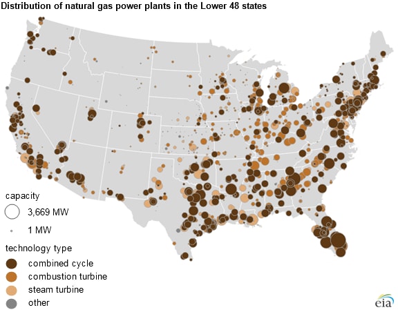
Via EIA.
The next largest category of water use is public water consumption. Because public water mostly consists of water used in homes, I’ve also included self-supplied water used by homes. The maps below show public and self-supplied water use by state.
!function(){"use strict";window.addEventListener("message",(function(e){if(void 0!==e.data["datawrapper-height"]){var t=document.querySelectorAll("iframe");for(var a in e.data["datawrapper-height"])for(var r=0;r<t.length;r++){if(t[r].contentWindow===e.source)t[r].style.height=e.data["datawrapper-height"][a]+"px"}}}))}();Because public and self-supplied water use is a function of population, this map is basically a population map. So let’s also look at public and self-supplied water use per capita.
!function(){"use strict";window.addEventListener("message",(function(e){if(void 0!==e.data["datawrapper-height"]){var t=document.querySelectorAll("iframe");for(var a in e.data["datawrapper-height"])for(var r=0;r<t.length;r++){if(t[r].contentWindow===e.source)t[r].style.height=e.data["datawrapper-height"][a]+"px"}}}))}();There’s less variation here than I expected. The highest consuming states (Utah, Idaho) use only about two times the amount of water per capita as the lowest consuming states.
If we look at self-supplied water use specifically, we can see that it's highly regionally concentrated. In some areas of the country, self-supplied water makes up nearly all domestic water use, while in other areas of the country it's much less common.
 Via Circle of Blue.
The next largest category of water use is industrial. The map below shows industrial water use by county:
!function(){"use strict";window.addEventListener("message",(function(e){if(void 0!==e.data["datawrapper-height"]){var t=document.querySelectorAll("iframe");for(var a in e.data["datawrapper-height"])for(var r=0;r<t.length;r++){if(t[r].contentWindow===e.source)t[r].style.height=e.data["datawrapper-height"][a]+"px"}}}))}();Industrial water consumption is concentrated in a very small number of locations: northern Indiana for steel production, Louisiana and the Gulf Coast for oil refining, and so on. 100 of the US’s 3200 counties are responsible for more than 70% of the US’s industrial water consumption, and 23% of US industrial water use is concentrated in just five counties.
Water use over timeHow have patterns of water consumption changed over time? Overall water use peaked in 1980, and has trended downward since then.
!function(){"use strict";window.addEventListener("message",(function(e){if(void 0!==e.data["datawrapper-height"]){var t=document.querySelectorAll("iframe");for(var a in e.data["datawrapper-height"])for(var r=0;r<t.length;r++){if(t[r].contentWindow===e.source)t[r].style.height=e.data["datawrapper-height"][a]+"px"}}}))}();Thermoelectric power use is down more than 37% from its peak, irrigation use is down 21%, industrial is down at least 43% (and probably more), and public plus self supplied domestic water use is down 12% in absolute terms and 22% in per-capita terms.3
!function(){"use strict";window.addEventListener("message",(function(e){if(void 0!==e.data["datawrapper-height"]){var t=document.querySelectorAll("iframe");for(var a in e.data["datawrapper-height"])for(var r=0;r<t.length;r++){if(t[r].contentWindow===e.source)t[r].style.height=e.data["datawrapper-height"][a]+"px"}}}))}();Another trend from the 1950s through the 1970s was increased use of groundwater. Between 1950 and 1980 the annual volume of groundwater used in the US more than doubled, from 34 billion gallons per day to 83 billion gallons per day. Since then, groundwater use has been roughly constant (as of 2015, it’s at 82.3 billion gallons per day), even as surface water use has declined by nearly 30%. Groundwater is thus making up an increasingly large fraction of overall water use.
!function(){"use strict";window.addEventListener("message",(function(e){if(void 0!==e.data["datawrapper-height"]){var t=document.querySelectorAll("iframe");for(var a in e.data["datawrapper-height"])for(var r=0;r<t.length;r++){if(t[r].contentWindow===e.source)t[r].style.height=e.data["datawrapper-height"][a]+"px"}}}))}();ConclusionMy overall takeaway is that you need to be careful when talking about water use: it’s very easy to take figures out of context, or make misleading comparisons. Very often I see alarmist discussions about water use that don’t take into account the distinction between consumptive and non-consumptive uses. Billions of gallons of water a day are “used” by thermal power plants, but the water is quickly returned to where it came from, so this use isn’t reducing the supply of available fresh water in any meaningful sense. Similarly, the millions of gallons of water a day a large data center can use sounds like a lot when compared to the hundreds of gallons a typical home uses, but compared to other large-scale industrial or agricultural uses of water, it's a mere drop in the bucket.
On the other hand, it’s also easy to go too far in the other direction. People sometimes invoke the idea that water moves through a cycle and never really gets destroyed, in order to suggest that we don’t need to be concerned at all about water use. But while water may not get destroyed, it can get “used up” in the sense that it becomes infeasible or uneconomic to access it. If we draw down aquifers that have spent hundreds or thousands of years accumulating water, the water isn’t “gone” in the sense that it's been chemically transformed back into hydrogen and oxygen, but much of it probably ends up in the atmosphere, the ocean, or other places not readily or cheaply retrievable. Outside of large-scale desalination of ocean water, we’re ultimately limited in how much fresh water we can use by the amount of precipitation we get, and while we currently use a very small fraction of total precipitation (around 6%), it’s not as if there’s no limit to how much naturally-produced fresh water is available.
1Evapotranspiration is the combination of evaporation and transpiration (water evaporating from plants).
2There’s something of a data inconsistency here. If you look only at states that give data for irrigated cropland specifically, it suggests that 95% or more of irrigation water is used for crops. However, overall irrigation water is on the order of 118 billion gallons of water a day, but sources like the USDA suggest that irrigated cropland is only around 70-75 billion gallons a day, leaving around 40% of irrigation water unaccounted for. It’s not clear to me whether irrigation water use is around 95% (and USDA is undercounting or USGS is overcounting), or if it's closer to 60% and there’s some other huge user of irrigation water.
3It’s hard to be sure about industrial since prior to 1980 it was lumped in with mining.
August 16, 2025
Reading List 08/16/25
 F22 Raptor engine exhaust, via @sci_fi_infra.
Welcome to the reading list, a weekly roundup of news and links related to buildings, infrastructure, and industrial technology. This week we look at efforts to stop solar and wind permitting, Ford’s new manufacturing process, Lake Powell’s water levels, Tesla’s used car prices, and more. Roughly 2/3rds of the reading list is paywalled, so for full access become a paid subscriber.
Some housekeeping items this week:
I’m going to try to keep the plugging to a minimum, but I’ll mention once more that my book, The Origins of Efficiency, is now available for preorder.
Some folks have asked about the high prices for international shipping for the book listed on Stripe’s website; for international orders your best bet is probably to just wait until the book is available on your country’s Amazon page.
I was on Marketplace briefly talking about shipbuilding again.
I was a guest on the World of DaaS podcast.
Solar and wind permitting and capacity densityThe US Department of the Interior is apparently still looking for ways to shut down wind and solar construction. A new order from the secretary, SO 3438, questions whether permitting wind and solar projects on federal land is even legal because of how much land they use. From the order:
This Order directs the Department of the Interior (Department), consistent with the Federal Land Policy and Management Act (FLPMA) and the Outer Continental Shelf Lands Act (OSCLA), to optimize the use of lands under its direct management, including the Outer Continental Shelf, (hereafter referred to collectively as “Federal lands”) by considering, when reviewing a proposed energy project under the National Environmental Policy Act (NEPA), a reasonable range of alternatives that includes projects with capacity densities meeting or exceeding that of the proposed project…Ultimately, FLPMA’s multiple use mandate for onshore lands, OCSLA’s multiple requirements for offshore activities, and NEPA’s requirement to consider reasonable alternatives to a proposed action give rise to the question on whether the use of Federal lands for any wind and solar projects is consistent with the law, given these projects’ encumbrance on other land uses, as well as their disproportionate land use when reasonable project alternatives with higher capacity densities are technically and economically feasible.
As Jason Clark of Power Brief notes, “capacity density” is basically a made-up metric created specifically to try and make wind and solar projects look bad, and is not even being applied consistently:
DOI is questioning if *any* wind or solar should be permitted (their emphasis on *any*).
It's all tied back to this new metric called "CAPACITY DENSITY" which is an invented formula to ding projects on a combo of:
1) Capacity Factor (hashtag#AgeofBaseload)
2) Acreage used for a lease
By DOI's estimations the holy grail of Capacity Density is a nuclear AP1000 project with a score of 33.17. In this case higher number = better.
DOI claims that solar, solar+storage, and wind are "too low" on this metric compared to other reasonable alternatives. Of course not accounting for varied capacity factors or multiple uses of land....
The Big Contradiction:
Everything is "low" compared to a nuclear facility -- even a Combined Cycle Natural Gas plant is nearly 9 points "worse."
But the cutoff for what is vs. what isn't an acceptable Capacity Density seems entirely arbitrary.
Take Coal and Geothermal. DOI has taken steps to ENHANCE the permitting for both -- even though their Capacity Density is pretty crappy compared to nuclear, SMRs, and all forms of Natural Gas generation.
There are a thousand other flaws in this…
Some other flaws in this are the fact that only a tiny fraction of the land “used” by a wind project is actually occupied by the turbines, and that land is massively more valuable when used to produce solar power than it would be if it were used for many other widely accepted purposes, such as growing corn. This is also another unfortunate example of how easily the tools of environmental review can be used to harm the environment.
Is air travel getting worse?At Maximum Progress, Max Tabarrok looked at every non-stop flight in the US since 1987 to determine if flight delays were getting worse. He found that short delays have actually gotten less common, but only because airlines have lengthened the scheduled travel times of flights to give themselves more padding. Long delays (in excess of 90 minutes), on the other hand, have increased by a factor of four:
Now we have some explanation for the pattern we saw above. Within the same routes, flights are now about 10 minutes longer than they were in 1987, partly reflecting more frequent delays pulling up average flight times and partly due to slower cruising speeds for fuel saving.
Starting around 2008, Scheduled flight times began increasing even faster than actual ones, and are now 20 minutes longer than their 1987 pairs along the same routes. This divergence makes it look like far more flights are early in 2024 when in reality almost all flights are taking longer.
Similarly, if take all the routes in the 2024 graph and compare the actual flight time to the scheduled flight time on that same route in 1990, we see that most flights in 2024 are late by 1990 standards.
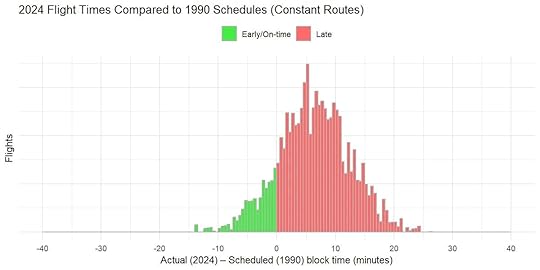

Max notes that adding 10 minutes to flights on average costs travelers around $6 billion a year, but I wonder if this change isn’t actually utility enhancing. Extending the scheduled trip time of flights, and thus making them longer but less likely to be late, probably means fewer missed connections, delayed meetings and other similar problems. Time spent traveling rises, but coordination failures decline, and the tradeoff might be worth it.
Ford goes unboxedIn September of last year, Tesla unveiled a novel car production process that it called “unboxed”. Rather than assemble the frame of the car and then attach components to it piece by piece on a conventional assembly line, the frame would be broken up into a series of large modules, each one built to a substantial level of completion before being attached together. Because less work would need to be done inside the already assembled car body, this would make the process more efficient. (We see a similar method of construction used in shipbuilding, adopted for similar reasons.)
Tesla has only partly begun to deploy its unboxed process, but it looks like Ford is going to attempt a similar production process for its new, low cost truck EV. Via Ars Technica:
3D printing advances
Ford is splitting the production line into three. One assembles the front subassembly, another the rear subassembly, and the third the battery pack and interior, which then meet for final assembly. And it's moved to large single-piece castings for the front and rear subframe to allow this approach.
"There are other people that use large-scale castings but not in the way we do. We know of no one that has ever built a vehicle in three parts in this way and brought it together at the end," explained Field. "So it really goes way beyond a typical modular architecture that existing manufacturers have out there," he said.
"I don't think there's any platform that has been so blank-slate, architected around having a large subassembly that you can put a whole bunch of parts on," added Alan Clarke, executive director of advanced EV development.
I’m always on the lookout for new, interesting manufacturing processes or capabilities, and I especially like seeing the boundaries of 3D printing/additive manufacturing being pushed. Here’s a paper where someone 3D printed an electric motor, using a special plastic that had iron fragments embedded in it. From the abstract:
This paper catalogues a series of experiments we conducted to explore how to 3D print a DC electric motor. The individual parts of the electric motor were 3D printed but assembled by hand. First, we focused on a rotor with soft magnetic properties, for which we adopted ProtoPastaTM, which is a commercial off-the-shelf PLA filament incorporating iron particles. Second, we focused on the stator permanent magnets, which were 3D printed through binder jetting. Third, we focused on the wire coils, for which we adopted a form of laminated object manufacture of copper wire. The chief challenge was in 3D printing the coils, because the winding density is crucial to the performance of the motor. We have demonstrated that DC electric motors can be 3D printed and assembled into a functional system. Although the performance was poor due to the wiring problem, we showed that the other 3D printing processes were consistent with high performance. Nevertheless, we demonstrated the principle of 3D printing electric motors.
And here’s a video describing a process called volumetric 3D printing. Conventional resin 3D printers use specific wavelengths of light to rapidly cure a light-sensitive resin layer by layer. Volumetric 3D printing uses a similar photo-sensitive resin, and rotates a container of it while projecting a specially-designed image onto it, which varies as the container rotates. As the light passes through the resin, it cures the resin in the shape of the object, printing it in just a few seconds.

August 12, 2025
My Book "The Origins of Efficiency" is Now Available for Preorder
I’m happy to announce that my book, The Origins of Efficiency, is now (officially) available for preorder, and will be released on September 23rd.1 You can preorder on Amazon, Stripe, Barnes and Noble, or Bookshop.com.
 Why I wrote this book
Seven years ago, I joined a well-funded, high-profile construction startup called Katerra. At the time I was a structural engineer with about ten years of experience, and over the course of my career I had become increasingly disillusioned with the inefficient state of the construction industry. Over and over again, engineers and architects were designing similar sorts of buildings, instead of building multiple copies of the same design. Contractors were putting up buildings on-site, by hand, in a way that didn't seem to have changed much in over a century.
Productivity statistics told much the same story: unlike productivity in other industries, like manufacturing or agriculture, construction productivity has been flat or declining for decades, and it’s only getting more expensive to build homes, apartments, and other buildings over time.
!function(){"use strict";window.addEventListener("message",(function(e){if(void 0!==e.data["datawrapper-height"]){var t=document.querySelectorAll("iframe");for(var a in e.data["datawrapper-height"])for(var r=0;r<t.length;r++){if(t[r].contentWindow===e.source)t[r].style.height=e.data["datawrapper-height"][a]+"px"}}}))}();Katerra had a plan for changing all that. It would efficiently build its buildings in factories rather than on-site, doing for construction what Henry Ford had done for cars. Katerra already had several factories in operation or under construction when I joined, and planned to build even more. At the time, I thought Katerra’s approach was exactly what was needed to change the industry. It seemed obvious that factory-built construction would be more efficient, but that some combination of incentives, inertia, and risk aversion kept the industry locked into using old, inefficient methods of production. I thought that with a sufficient jolt, the industry could be disrupted and new, better ways of building could take root. Katerra had raised over $2 billion in venture capital to supply that jolt.
But within a little over three years, Katerra had burned through all its venture capital, gone through increasingly brutal rounds of layoffs (one of which cut the engineering team I was leading by around 75%), and declared bankruptcy. I survived the layoffs, but had left the company several months before its final end. When Katerra closed its doors, I was working at a new engineering job, back to designing the same sort of buildings, built using the same old methods I’d used for most of my career.
Since then, the construction industry hasn’t improved its track record of productivity. In fact, post-Covid, construction costs had one of their steepest rises in history.
As Katerra was collapsing, I became obsessed with understanding why things had gone so wrong, and what it would take to actually make the construction industry more efficient. I started writing Construction Physics just after I left the company, as a way to work through an understanding of how the construction industry worked and why Katerra had failed to change it.
Some of Katerra’s failure can be blamed on operational missteps: trying to develop too many products at once before finding product-market fit, failing to integrate acquired companies, and so on. But it also gradually became clear that Katerra’s fundamental thesis — that construction would be much cheaper and more efficient if it was done in factories — was either incorrect, or woefully incomplete. Time and again at Katerra, the engineering team would design some new factory-produced building, only for the costs to come back too high. Time and again executives would complain how hard it was for Katerra, with its expensive factories and high overheads, to compete against “Bubba and his truck,” who could put up buildings using little more than hand tools. Rather than enabling radically cheaper construction, as Ford’s assembly line had done for the Model T, Katerra’s factories were making it hard to even compete in the existing market.
It also became clear that Katerra was far from the first company to try and fail to transform the industry using factory-built construction. I learned that such attempts stretch back decades: from the Lustron Corporation in the 1940s, to Stirling Homex and the other Operation Breakthrough companies in the 1960s, to Veev in the 2020s. Often these companies failed as quickly as Katerra did. Other times, they managed to carve out successful businesses: National Homes successfully built prefab homes for nearly 50 years. But no one had managed to use prefab to become the Henry Ford of housing.
And the problem didn’t seem limited to the US. While prefab, factory-built construction is often much more popular in other countries than it is in the US, nowhere did I find it ushering in dramatic cost reductions. Toyota, arguably one of the best manufacturers in the world, formed a prefab housing company in Japan in the 1970s to apply its manufacturing expertise to homebuilding. But while in car manufacturing Toyota was so efficient and successful that it eventually set the global standard, Toyota remains a niche player in homebuilding, and its homes are surprisingly expensive compared to site-built construction.2 In Sweden, nearly all single-family homes are factory-built, but their construction costs are higher than conventionally-built homes in the US.
It eventually became clear to me that we didn’t really understand what it took to make some process more efficient. Those of us hoping to use factory-built construction to drive down costs were acting as a sort of cargo cult — duplicating what we saw work elsewhere, without truly understanding the mechanisms that made the process successful. To understand why the construction industry was so resistant to efficiency improvements, and why it never seemed to get cheaper to construct buildings, I needed to understand how, specifically, things get cheaper to produce over time.
This book is the fruit of that effort.
Over the course of roughly a year and a half, I looked at dozens of production processes — from cigarette making to package delivery, from steel production to tomato harvesting — to see how they improved over time. I read about the history of virtually every industrial improvement system: from scientific management to Lean production, from DFMA to SMED, from Taguchi methods to statistical process control. I read the work of economic historians who had studied industrial progress like Joel Mokyr, Alfred Chandler, David Hounshell, Gregory Clark, Sam Hollander, and John Enos. I bought lots and lots of books. The bibliography of the book has around 600 separate references, and on its own would be one of the longest pieces of text I’ve ever produced. (Writing this book is what forced me to start using proper reference management software.)
I initially thought that turning all this reading into a book would be essentially the same process as writing the newsletter. At the time, my newsletters averaged around 2,000 words each, and I estimated that the book would be around 100,000 words, or require around 50 newsletters’ worth of work. But I was sorely mistaken. It turns out that it's comparatively simple to write 50 stand alone pieces of text that collectively add up to the length of a book. Tying many disparate ideas into a single, coherent thesis, and then explaining that thesis via separate chapters that draw on and reference each other, is much more complex. (This is why you see so many books which are loose collections of thematically similar chapters: it’s much easier to write that sort of book.)
Over the course of writing the newsletter I had developed a writing process that worked very well, but this process was ill-suited to produce a book-length work. Once I signed the contract with Stripe Press, I thought I’d immediately able to start cranking out chapters, but for roughly six months I struggled to produce anything useful (there were multiple times when I sent a draft chapter to someone, then quickly followed up with “Don’t read that, it’s trash,” and started over).
Writing the newsletter is essentially a linear process: I read everything I can on a topic, take note of the especially interesting or relevant facts and information, and then come up with a structure for an essay that can incorporate it all. Once this structure is in hand, it's simply a matter of expanding the basic structure into a draft, and a draft into the final version. For the book, I eventually figured out that I needed to turn this linear process into a cyclical one. Instead of going from reading to structure to draft to final version, I would read, come up with some tentative ideas for a structure, then use those ideas to guide further reading, repeating the process until I felt like things had “clicked” and my structure was robust. Only then could I start fleshing out the basic ideas into a draft.
After several months of this, I was able to condense down the mass of information I had collected into a relatively simple framework: a small number of specific things you can do to make a process more efficient.
The book is 10 chapters, plus an introduction and conclusion. Chapter 1 explains this basic framework: the structure of a production process and the options you have for making it more efficient. Chapters 2 through 6 explain each one of these strategies, drilling into the details and nuances of how they work, when they don’t work, and examples of how they’ve reduced costs or improved operations in actual production processes. Chapters 7, 8, and 9 explain how these various strategies can work together and reinforce each other, collectively creating enormous efficiency improvements. Chapter 10 explains what happens when these paths to efficiency improvement are blocked, using the construction industry as an example.
I’m immensely proud of this book; if it sounds interesting or valuable to you, I hope you’ll pre-order it.
1It’s technically been listed on Amazon for months, but only recently have the cover and everything else been finalized.
2August 9, 2025
Reading List 08/09/2025
 Guangzhou Circle, Guangzhou, China, via @sci_fi_infra.
Welcome to the reading list, a weekly roundup of news and links related to buildings, infrastructure, and industrial technology. This week we look at microplastics in the air, the Blanchard lathe, the report on the OceanGate sub disaster, a plan to visit a black hole, and more. Roughly 2/3rds of the reading list is paywalled, so for full access become a paid subscriber.
Some housekeeping items:
IFP is partnering with Matt Yglesias to solicit ideas for improving federal mass transit policy. If you have an idea for improving mass transit policy, submit a proposal here.
I had planned to publish a piece on the nature of technological progress this week, but it didn’t quite come together the way I hoped, so I’m currently reworking it.
SpinlaunchRockets are a difficult way of putting objects into space. In addition to the technological difficulties inherent in controlling an exploding river of hot gasses, rockets have the unfortunate property that each additional bit of mass launched requires more fuel to lift it, which then requires more fuel to lift that fuel, and so on (a mechanism described as the tyranny of the rocket equation). The result is that rocket payload fractions are a single digit percent of total rocket mass.
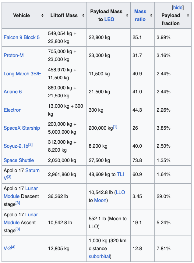 Via Wikipedia.
There’s thus perennial interest in finding ways to put objects into orbit other than using rockets. One such idea is to use a huge gun to launch a projectile into orbit. This idea has a long history (it’s used to launch a spacecraft in Jules Verne’s 1865 From the Earth to the Moon), and there have been various attempts to build a gun that could launch a projectile into space.
A current attempt to launch a projectile into space is Spinlaunch which, per the name, wants to launch satellites using a huge centrifuge. (This doesn’t completely eliminate the need for a rocket, but will apparently greatly reduce the fuel requirements.) Wired has a long profile of the company:
Ozimek on the US car industry
The idea that an object weighing thousands of pounds can punch its way into space after spinning in circles on Earth’s surface can be hard to fathom. It might even sound crazy, and the company has a lot to prove to shake its critics. So far it has managed to spin an 11-pound dummy payload at more than 4,000 mph and send it crashing into a steel wall. Between those tests and the edge of space, however, are roughly a hundred miles and a whole lot of air resistance. Never mind the engineering work needed to build a centrifuge 100 yards wide, with an arm strong enough to support a roughly SUV-sized rocket.
Yaney hopes this is the year he achieves vindication. The company plans to conduct its first suborbital launches this winter at a new test site in New Mexico. Assuming the system works, Spinlaunch promises to reduce the cost of sending small satellites into space by a factor of almost 20. But the bigger deal may be its launch cadence. Yaney predicts the mass accelerator will be able to do five launches a day; most rocket companies can’t do that many launches in a month. In the era of mega-satellite constellations, which will see thousands of small satellites sent to low Earth orbit over the next decade, Yaney believes Spinlaunch’s time has come.
Adam Ozimek of the Economic Innovation Group has an interesting paper on the evolution of the US auto industry, and whether it needs protection from foreign competition. Among other things, he argues that despite common perception, the industry hasn’t collapsed: output has been steady by number of cars and has greatly increased by value add. Rather, it was Detroit specifically that collapsed, as car manufacturers moved production to elsewhere in the US:
The historical record paints the picture. Henry Ford II announced in 1950 that his company’s investments would no longer be concentrated in their established industrial centers. By the mid1960s, Ford had made major investments not just in the southern states of Alabama, Tennessee, and Georgia, but also in New York and New Jersey.
For its part, GM made investments in Indiana, Ohio, Illinois, New Jersey, Mississippi, and
California, while Chrysler invested in New York, Delaware, Indiana, and Ohio — all by the late 1950s.
These investments and the jobs that followed them did not occur as a result of foreign car companies establishing their factories in the south and other parts of the country. That came much later. Long before the Big 3 were seriously challenged by foreign automakers, they themselves had begun decentralizing auto investment out the industrial hub of Michigan and spreading jobs and investment across the rest of the country.
So globalization couldn’t kill Detroit because Detroit was already dead. Or at least dying.
And it really was a story of decline in Detroit almost exclusively. From 1950 to 1980, auto
employment even in most of the Rust Belt states expanded. The gains in Ohio, Indiana, and Illinois exceeded those of any southern state.
 Air microplastics
An occasional topic of interest around here is indoor air quality: I’ve previously written about how UV light could be used to help prevent future pandemics by killing airborne pathogens, and whether there are negative cognitive effects from carbon dioxide.
This PLOS ONE paper has put another indoor air pollutant on my radar: microplastics. From the abstract:
The ubiquitous presence of airborne microplastics (MPs) in different indoor environments prompts serious concerns about the degree to which we inhale these particles and their potential impact on human health. Previous studies have mostly targeted MP in the 20–200 µm size range, which are less likely to efficiently penetrate into the lungs. In this study, we specifically investigate airborne, indoor suspended MPs in the inhalable 1–10 µm (MP1–10 µm) range in residential and car cabin environments, by using Raman spectroscopy. The median concentration of total suspended indoor MPs for the residential environment was 528 MPs/m3 and 2,238 MPs/m3 in the car cabin environment. The predominant polymer type in the residential environment was polyethylene (PE), and polyamide (PA) in the car cabin environment. Fragments were the dominant shape for 97% of the analyzed MPs, and 94% of MPs were smaller than 10 µm (MP1–10 µm), following a power size distribution law (the number of MP fragments increases exponentially as particle size decreases). We combine the new MP1–10 µm observations with published indoor MP data to derive a consensus indoor MP concentration distribution, which we use to estimate human adult indoor MP inhalation of 3,200 MPs/day for the 10–300 µm (MP10–300 µm) range, and 68,000 MPs/day for MP1–10 µm. The MP1–10 µm exposure estimates are 100-fold higher than previous estimates that were extrapolated from larger MP sizes, and suggest that the health impacts of MP inhalation may be more substantial than we realize.
Note that I haven’t read this paper closely, and these sorts of findings sometimes turn out to be overblown or incorrect. (Cremieux notes, for instance, that a widely-referenced paper blaming asthma on gas stoves turned out to be incorrect.) But particles in the air will in general cause health problems, so if there are many more plastic particles in the air than previously realized that seems likely to be bad.
Blanchard latheIf you read much on the history of American invention, you’ll quickly come across mention of the Blanchard lathe, a clever invention made in the early 19th century for manufacturing gunstocks. The lathe used an existing gunstock as a cam mechanism: as the existing gunstock rotates, it pushes against a movable arm connected to a saw. The path of the saw movement matches the shape of the existing gunstock, and can cut a piece of wood into the same shape.
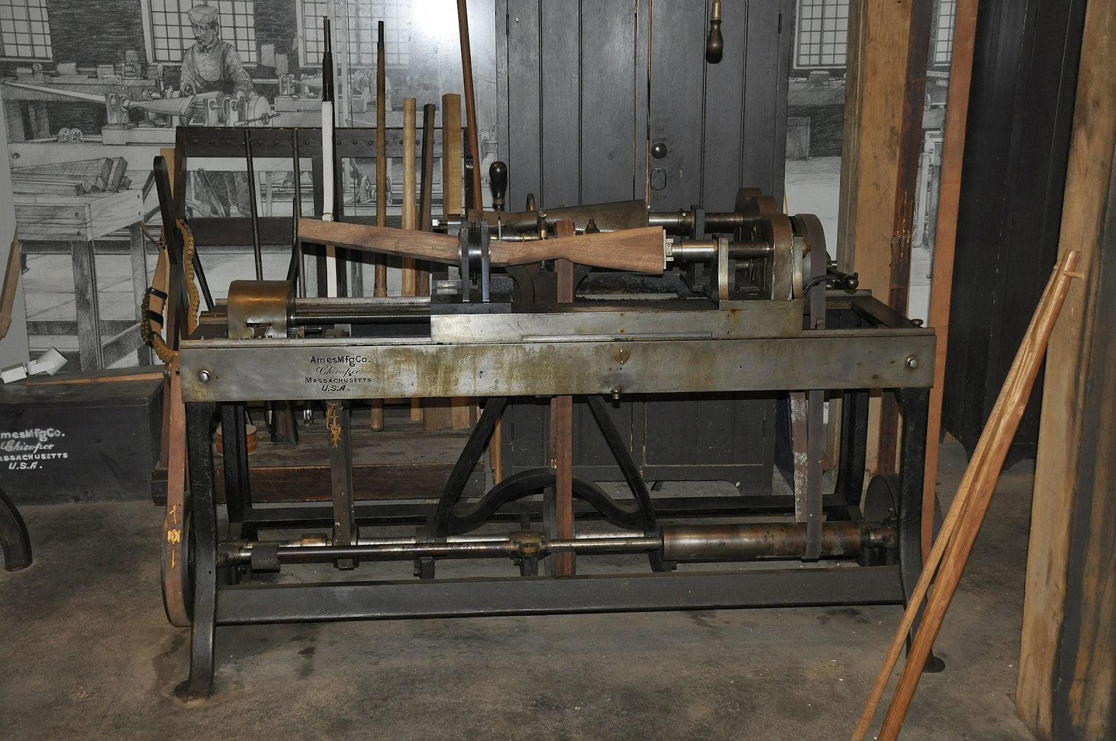 Blanchard lathe, via Wikipedia.
Most discussions of the lathe only mention its invention, but apparently such lathes remained in use well into the 20th century. On Twitter, hw97karbine posts a video of a Blanchard lathe being used to manufacture the stock for a German Karabiner 98k around 1939.

August 7, 2025
Group Technology, the Forgotten Cousin of Lean Manufacturing
Industrial improvement systems — strategies for making a business more profitable, more efficient, or better operated — rise and fall in popularity over time. Today, the most widely known improvement systems are probably various flavors of “Lean methods," the adaptation of the Toyota Production System first made popular by the 1990 book The Machine that Changed the World. But go back to the 1950s, and efficiency experts will instead tout the benefits of “work simplification," a collection of strategies for streamlining production processes and eliminating wasteful or unnecessary steps. (Work simplification is still occasionally recommended as a method of process improvement today, including by the consultant with the unfortunate website URL www.worksimp.com.) Go even farther back to the turn of the century, and the dominant improvement strategy will now be Frederick Taylor’s scientific management.1
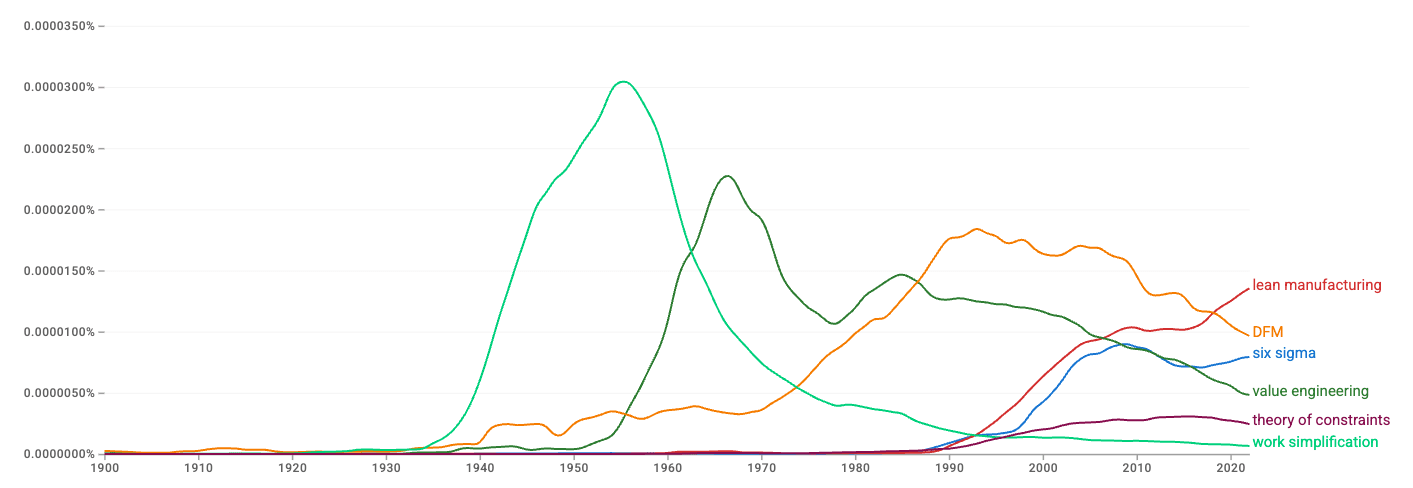 Frequency that different industrial improvement systems are mentioned in books via Google Ngram Viewer.
One lesser known industrial improvement system that appeared and then receded in the second half of the 20th century is Group Technology. Group Technology first arose in the Soviet Union, and shares many similarities with Lean methods. But its popularity peaked in the 1980s, and today it seems mostly forgotten. It’s interesting to try and understand what made it seem compelling, and why it ultimately lost favor.
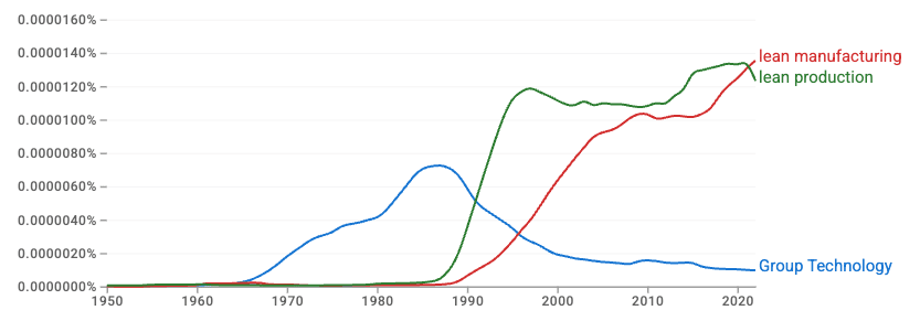 Frequency that different industrial improvement systems are mentioned in books via Google Ngram Viewer.Premise of Group Technology
Group Technology is an improvement system designed to apply to factories, machine shops, or other production operations that produce a wide variety of different parts in relatively small numbers. Unlike mass production, which can use dedicated production lines to produce large volumes of identical or near-identical goods, equipment in these high-mix, low-volume operations will be used to produce a variety of different parts or components depending on the day. A machine might be used for Part A today, Part B tomorrow, Part C the next day, and so on.
The basic idea behind Group Technology is that many of the parts and components produced in these sorts of operations will share similarities. A machine shop might make 50 different types of steel bolt, depending on the exact product or the customer’s order, but while the sizes and shapes of the bolts might differ, they’ll likely all use similar materials and require the same sort of operations done in roughly the same order. These similarities can be exploited to make production operations more efficient. In Group Technology, similar parts made from similar materials and that require similar operations are grouped together (hence the name), and produced in manufacturing cells dedicated to those types of parts. These cells contain the exact machines needed, arranged in the order that they’re needed and configured to do the sorts of jobs that the parts require.
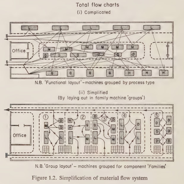 Types of factory layout, via “The Introduction of Group Technology”.
This arrangement yields several benefits:
Movement and travel times are reduced. Parts don’t need to be routed all over the factory, but move quickly through a series of machines dedicated to particular groups.
Setup times are reduced. Machines can be configured to quickly perform the sorts of operations a particular group of parts or components requires.
Work in process and cycle times are reduced. With less movement and setup time, products get routed through the necessary steps much more quickly, resulting in less inventory piling up and products getting to the customer much faster. Short cycle times allow for material to be ordered frequently in smaller batches, paced to the level of demand, making it easier to flexibly respond to market changes.
Capital costs are reduced. Less work in process means smaller factories are required, and reduced setup times results in greater equipment utilization, squeezing more output from a given amount of equipment.
More generally, Group Technology aims to achieve many of the benefits of mass production in a high-mix, low-volume production operation.
A brief history of Group TechnologyThe basic ideas behind Group Technology — creating dedicated production areas for similar sorts of parts — began to emerge in the early 20th century in the wake of mass production, assembly line methods.2 In 1925, American engineer RE Flanders described a method of production control which emphasized “standardization of product, departmentalization by product rather than process, minimized transportation, visual control of work itself instead of remote control by records.’” In 1938, JC Kerr, another American engineer, described grouping machine tools together to “smooth the flow of production as it does in a one-product shop.” And in 1949, Swedish engineer Arn Corling described the reorganization of a Swedish bus manufacturer around principles of what he called “group production”:
He wrote that group production was an adaptation of line production to the machine shops working on batch production and that “this implies radical decentralisation into small independent production units or groups, each comprising the machines and everything needed for the complete manufacture of a special category of parts.”
But it was the Soviet Union where Group Technology as a holistic system of improvement truly emerged. In 1937 Soviet professor AP Sokolovskiy suggested that “parts of similar configuration and features should be manufactured by standard processes, thus making it possible to introduce flow line into batch production.” In 1952, Soviet engineer SP Mitrofanov published a monograph on using ideas of group production on turret lathes, and began consulting with other factories on how the ideas could be adopted. Thanks to Mitrofanov’s efforts (he published four books on what he began to call Gruppovaya Tekhnoiogiya, or Group Technology, between 1955 and 1959), Group Technology began to gain traction in the USSR. Mitrofanov was awarded the Lenin Prize in 1959, and Group Technology was recommended by the Central Committee of the Communist Party. Group Technology became “one of the fashionable new technologies," and it was discussed frequently in seminars and talks. By the early 1960s, Group Technology was being used in hundreds of Soviet factories.
!function(){"use strict";window.addEventListener("message",(function(e){if(void 0!==e.data["datawrapper-height"]){var t=document.querySelectorAll("iframe");for(var a in e.data["datawrapper-height"])for(var r=0;r<t.length;r++){if(t[r].contentWindow===e.source)t[r].style.height=e.data["datawrapper-height"][a]+"px"}}}))}();As it spread in the Soviet Union, Group Technology also began to take root in Europe and the US. This seems to have been partly due to broader interest in codification and classification systems that were being developed in the late 1950s and early 1960s, and partly due to Mitrov’s book The Scientific Principles of Group Technology being translated into English in 1966. A conference on Group Technology was held in London in 1961, and it was discussed at a series of international conferences on classification and coding that were held in the 1960s. By the 1970s, there were at least half a dozen books published in English that touted the benefits of Group Technology, and companies like Boeing had adopted the methods in at least some form.
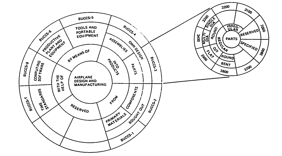 Boeing’s Group Technology-based BUCCS part classification system.
The peak of Group Technology’s popularity seems to have been the 1980s.3 Up through the end of the decade, it continued to be the subject of dedicated books, and merit substantial mentions in books on adjacent subjects (such as just-in-time and flexible manufacturing systems). But interest in the system seems to have rapidly fallen off in the 1990s.
!function(){"use strict";window.addEventListener("message",(function(e){if(void 0!==e.data["datawrapper-height"]){var t=document.querySelectorAll("iframe");for(var a in e.data["datawrapper-height"])for(var r=0;r<t.length;r++){if(t[r].contentWindow===e.source)t[r].style.height=e.data["datawrapper-height"][a]+"px"}}}))}();One industry that did, and (as far as I’m aware, still does) enthusiastically adopt Group Technology is shipbuilding. Modern texts on shipbuilding, such as Storch’s Ship Production, still make extensive reference to Group Technology as the system used to divide up work on a ship and in a shipyard. However, it’s not 100% clear to me when this “adoption” actually took place. From what I can see, it wasn’t until the late 1970s, when the US began studying modern shipbuilding methods in countries like Japan via the National Shipbuilding Research Program, that the label of Group Technology began to be applied. Researchers then retroactively described these methods as “working off the logic of Group Technology.”
Why interest in Group Technology wanedIt’s not 100% clear why interest fell in Group Technology, but I have some suspicions. Many of the valuable aspects of Group Technology — using manufacturing cells, reducing work in process and cycle times, eliminating wasteful part movements, decreasing setup times, increasing machine utilization — weren’t unique to group technology, but were similarly advocated by other industrial improvement systems like Lean methods and the Theory of Constraints. (Those familiar with Lean methods will note how similar the advertised benefits of Group Technology are to Lean.) And other systems often bundled these benefits into a much sexier package. Lean methods were spread by The Machine that Changed the World, a popularization of Womack and Jones’ academic research on the Japanese Auto industry, which sold in enormous numbers, like The Goal. Both of these books encapsulate their recommendations into an easily digestible format.
 Group Technology part codification system, via “Group Technology: Foundation for Competitive Manufacturing”
By contrast, what’s notable to me when reading about Group Technology is how much emphasis is immediately placed on the tedious process of part coding and classification. It often seems like developing a part coding scheme and the necessary documentation (which might entail creating thousands of new part drawings) is the main thing Group Technology efforts end up focusing on. A 1989 survey of US Group Technology users, for instance, extensively discusses the codification schemes and issues with implementing them, but makes no mention of any benefits achieved in terms of reduction of part movement, setup or cycle times, or machine efficiency (the only benefits discussed relate to part design and process planning). Often this codification seems to have involved buying some off the shelf codification system (along with implementation software), and then adapting it to the needs of the specific business.
Given how much emphasis it places on doing tedious paperwork and software configuration, it’s not surprising to me that there were no breakout Group Technology hits like The Goal or The Machine That Changed The World, or that systems that repackaged many of Group Technology’s basic ideas, without the immense emphasis on paperwork, became more successful.
1Scientific management isn’t shown on this graph, but its early 20th century peak is much higher than any subsequent peaks, and even following its decline it still has more frequent mentions than any other system. I suspect this is due to interest as a subject of historical study.
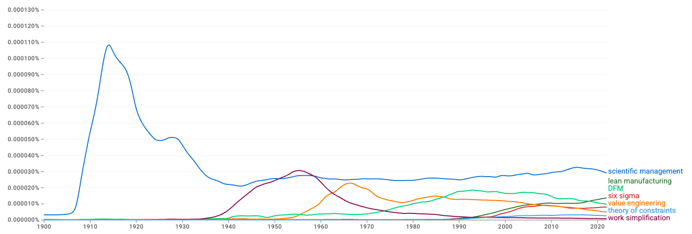 2
2It was likely the adoption of electricity, which allowed machine tools to have their own dedicated electric motors, which made Group Technology possible. Prior to dedicated electric motors, machines were driven by belts connected to overhead drive shafts, which limited flexibility in machine arrangement. Giving each machine its own motor removed this constraint. (industrial innovation in the soviet union 106).
3In general, the 1980s seem to have been a period of high demand for industrial improvement systems, possibly due to falling US competitiveness compared to foreign countries like Japan. In addition to books on Group Technology appearing that decade, Goldratt published The Goal, his bestselling business novel describing the Theory of Constraints. The 1980s is also when interest in Japanese manufacturing techniques really began to take off.
August 2, 2025
Reading List 08/02/2025
 Goddess of Kannon statue, Japan, via @sci_fi_infra.
Welcome to the reading list, a weekly roundup of news and links related to buildings, infrastructure, and industrial technology. This week we look at European multifamily construction, a robot lamp, China’s self-driving car test, a “mini Moravec’s paradox”, and more. Roughly 2/3rds of the reading list is paywalled, so for full access become a paid subscriber.
No essay this week, but I’m working on a more involved piece about the nature of technological progress that should be out next week.
Housing monopoliesA line of argument I haven’t been paying much attention to but has (apparently) been gaining traction is the idea that recent increases in housing costs are driven by monopolies in homebuilding. This theory has been advanced by folks like Matt Stoller, but evidently it's gaining currency with others as well.
This theory didn’t seem completely crazy to me, as over the past several years homebuilding has steadily gotten more concentrated. It used to be that the 10 largest homebuilders were responsible for a very small fraction of total homes built in the US, but today they’re responsible for an increasingly large share. But I had never really looked into the idea.
However, a good piece by Derek Thompson on his substack lets some air out of this theory:
European multifamily construction
It is a fact that home prices across the country have increased in the last decade. It is also a fact that homebuilders have gotten bigger in the last few years. The question at stake here is: Is the second fact causing the first fact?
I believe there is only one economic paper that unambiguously says yes. It is a 2023 working paper entitled “Fewer players, fewer homes: concentration and the new dynamics of housing supply” by the economist Luis Quintero. This research is load-bearing in the antitrust world. It’s quoted in articles and social media posts by the antitrust advocate Matt Stoller. You’ll find it in research from other antitrust scholars. And it seems to be the only empirical research in Musharbash’s essay.
I called Luis Quintero to ask what level of market concentration in homebuilding he considered to be dangerous. In the most concentrated markets, Quintero said, one or two firms account for 90 percent of new housing. But problems begin to accelerate, he said, if five or six firms account for 90 percent of new housing.
…I tracked down a complete listing of the country’s 50 largest homebuilding markets, from #1 Dallas to #50 Cincinnati. How many meet Quintero’s first oligopoly threshold (two companies = 90 percent of the market)? Zero out of 50. And how many meet his second threshold (six companies = 90 percent of the market)? One: Cincinnati. It turns out that the largest homebuilding markets just aren’t that concentrated, even when you accept the yardstick of the economist who’s offered the only empirical definition of market concentration in homebuilding that I can find.
It’s become clear that for many types of construction, European countries have much lower construction costs than the US does. Transit and subway construction is the most famous example of this, but it's my sense that in multifamily apartment construction, Europe is also often substantially cheaper.
With transit construction, some of this comes down to improved efficiency and lower labor costs, but some of it comes down to differences in what gets built: US transit apparently often has much larger, more expensive stations than European transit. It seems like something similar might be true for multifamily construction as well. On Twitter, developer Brendan Whitsitt looks at a recent multifamily project in Paris, and lays out the many differences which allow it to be built for less than a similar project in Canada (which I believe will be fairly similar to US requirements.)
 Robot lamp
I’ve spent a bit of time discussing humanoid robots, and considering whether a humanoid form factor will win out, or if other robot form factors might make more sense. In that vein, here’s a company developing a robotic floor lamp, Lume, that will (supposedly) autonomously fold clothes for you when it's released in 2026:

It’s not clear how close they are to an actual working robot (the video is entirely simulated, and I’d be surprised if they end up using a form factor that has so many joints/degrees of freedom), but if this seems compelling, you can place a reservation for the lamp here.
Elon Musk’s self driving car predictionsTesla has been working on self-driving cars since at least 2013, and has been shipping Autopilot hardware since at least 2014. Over the years, Elon Musk has frequently made predictions about when various self-driving capabilities will be available, which have reliably proved to be overly optimistic. Wikipedia has a helpful list of every prediction Elon Musk has made around self-driving cars, and the status of that prediction.

The list includes 29 predictions in total. Of these, 1 has been met, 3 have been partially met, 7 might still be met but haven’t yet, and 18 haven’t been met.
Brian Potter's Blog

- Brian Potter's profile
- 2 followers

